library(dplyr)  # data manipulation
library(purrr)  # functional programming
library(ranger)  # random forests
library(tictoc)  # performance timing
library(staccuracy)  # performance metrics
library(rsample)  # cross-validation

# Other packages accessed with :: direct access but not loaded (install them if needed):
# * stringr: string processing
# * readr: input CSV files
# * tidyr: data manipulation
# * cli: command line interface printing

# Accumulated Local Effects: ale package
# Install the development version of ale for this workshop, which is more recent than the current CRAN version.
# If needed, first install the pak package manager to easily install a GitHub package:
# install.packages('pak')
# pak::pak('tripartio/ale')
library(ale) # load the ale package only after installing the development versionAnalyzing a Large Corn Yield Dataset with ALE-Based Inference
February 17, 2026
Source:vignettes/ale-acdc-corn.qmd
1 Introduction
In this article, we analyze the Agro-Climatic Data by County (ACDC) dataset (Yun & Gramig 2017, licensed CC-BY), a county-level panel for the 48 contiguous U.S. states spanning 1981–2015, designed for agricultural production and climate research. It combines crop yields with key agro-climatic drivers, notably growing season degree days, total precipitation, and major soil characteristics, all preprocessed to focus on agricultural production areas.
Our focus here is predicting county-level corn yield per year (measured in bushels per acre) and then interpreting the factors that contribute to this prediction. The dataset’s structure matches the standard agro-climatic production framing, where output depends on temperature, precipitation, soils, and other controls.
2 Setup R environment
We begin by loading the packages used throughout the analysis. If any are not installed locally, the next step is to install them before running the rest of the document.
Note that the {ale} package is on CRAN, but for a few features used here we install the current development version from GitHub (the code shows how, via {pak}).
# For speed, these examples use retrieve_rds() to load precreated objects
# from an online repository.
# To run the code yourself, execute the code blocks directly.
serialized_objects_site <- "https://github.com/tripartio/ale/raw/main/download/corn_objects"
3 Dataset: ACDC corn yields
3.1 Corn data preparation
We work with the Agro-Climatic Data by County (ACDC), 1981–2015 (Yun & Gramig 2017). Rather than reproducing the full compilation code here, we summarize the key transformations used to assemble the analysis-ready dataset.
The ACDC data arrive in several components and require harmonization. First, agricultural land area is reported on grids measured in different years. We normalize these measures to the county-year level and express agricultural land area as square kilometres (ag_km2).
Temperature is the most involved transformation. ACDC stores temperatures as counts of days falling within one-degree Celsius bins (e.g., 2–3°C, 4–5°C, etc.). For modelling, we aggregate these bins into temperature ranges that are meaningful for corn (maize) growth, creating variables that count, for each county-year, how many days fall within each selected range. The data description below defines these ranges and notes why they are agronomically relevant.
When defining “in-season” windows, we restrict attention to months that align with typical crop calendars. The table below records the windows used in this analysis (initially chosen based on quick background guidance).
| Crop | Recommended Window |
|---|---|
| Corn | Mar–Aug |
| Soybean | Mar–Aug |
| Cotton | Apr–Oct |
| Wheat | Usually Apr–Oct (but depends if winter vs spring wheat) |
Soil composition variables come from county-level surveys conducted in 1992, 2001, 2006, and 2011. We carry those soil attributes forward to the county-year panel and merge them with annual corn yield, measured as bushels per acre (corn). Because this is a U.S. dataset, we report values in bushels per acre and provide a metric conversion alongside them.
After assembling the dataset, we inspect its structure (e.g., with glimpse()) to verify variable types and to see sample rows. We also compute summary statistics (min, max, mean, and interquartile values) for each variable. All variables used here are numeric; the next section defines each variable explicitly. The outcome of interest is corn, the corn yield (bushels per acre) for a given county in a given year.
3.2 Data description
corn_data |> glimpse()Rows: 90,010
Columns: 22
$ stco <fct> 1001, 1003, 1005, 1009, 1011, 1013, 1015, 1019, 1021, 1023,…
$ year <int> 1981, 1981, 1981, 1981, 1981, 1981, 1981, 1981, 1981, 1981,…
$ corn <dbl> 17.3, 101.4, 37.9, 53.8, 22.1, 50.5, 46.6, 65.5, 31.8, 45.9…
$ ag_km2 <dbl> 317.4507, 1000.1241, 429.0003, 447.9057, 266.2884, 187.1748…
$ temp_lt_00 <dbl> 1.252724e-03, 1.334438e-04, 2.644859e-02, 5.219093e-01, 2.0…
$ temp_00_10 <dbl> 9.108736, 5.825083, 9.556071, 16.302810, 10.703252, 9.11353…
$ temp_11_20 <dbl> 42.16270, 37.20385, 42.41642, 46.73110, 43.30999, 41.31729,…
$ temp_21_30 <dbl> 94.14356, 104.18624, 93.96831, 92.51842, 91.61782, 94.43539…
$ temp_31_35 <dbl> 34.43768, 35.64974, 34.00982, 26.71666, 34.06262, 34.72649,…
$ temp_36_45 <dbl> 4.14606767, 1.13495440, 4.02292888, 1.20910496, 4.28570742,…
$ temp_gt_45 <dbl> 0, 0, 0, 0, 0, 0, 0, 0, 0, 0, 0, 0, 0, 0, 0, 0, 0, 0, 0, 0,…
$ ppt <dbl> 620.8656, 679.8329, 567.0682, 652.4704, 551.0441, 540.4134,…
$ whc <dbl> 24.78343, 23.53884, 21.48367, 18.28257, 22.58728, 24.71647,…
$ sand <dbl> 59.68140, 59.09199, 61.74435, 37.50056, 39.39067, 50.83622,…
$ silt <dbl> 20.04843, 21.80517, 16.41010, 33.40470, 25.92334, 21.17595,…
$ clay <dbl> 20.27016, 19.10284, 21.84554, 29.09474, 34.68599, 27.98784,…
$ om <dbl> 111.80678, 185.66755, 88.42968, 79.91542, 120.90292, 71.662…
$ kwfactor <dbl> 0.2230648, 0.2503898, 0.2123219, 0.2454282, 0.2304381, 0.21…
$ kffactor <dbl> 0.2263995, 0.2561335, 0.2123997, 0.2962476, 0.2328219, 0.21…
$ spH <dbl> 5.139626, 4.940044, 5.127343, 4.914515, 5.529810, 5.031030,…
$ slope <dbl> 51.03629, 106.22105, 65.98003, 32.14657, 46.05617, 63.86830…
$ tfactor <dbl> 4.950716, 4.936530, 4.926214, 3.174986, 4.988563, 4.889981,…
corn_data |> summary() stco year corn ag_km2
1049 : 45 Min. :1981 Min. : 0.0 Min. : 0.4806
1077 : 45 1st Qu.:1988 1st Qu.: 80.0 1st Qu.: 316.7863
1079 : 45 Median :1993 Median :105.0 Median : 663.9057
1083 : 45 Mean :1995 Mean :106.0 Mean : 767.3234
1089 : 45 3rd Qu.:2002 3rd Qu.:131.9 3rd Qu.:1076.1543
5021 : 45 Max. :2015 Max. :238.8 Max. :5242.2723
(Other):89740
temp_lt_00 temp_00_10 temp_11_20 temp_21_30
Min. : 0.000 Min. : 0.000576 Min. : 8.025 Min. : 10.85
1st Qu.: 1.006 1st Qu.:19.224752 1st Qu.: 47.998 1st Qu.: 65.89
Median : 4.248 Median :29.188436 Median : 55.020 Median : 77.60
Mean : 6.241 Mean :27.847689 Mean : 54.521 Mean : 77.61
3rd Qu.: 9.698 3rd Qu.:37.250469 3rd Qu.: 62.071 3rd Qu.: 89.24
Max. :52.734 Max. :68.807006 Max. :131.138 Max. :128.56
temp_31_35 temp_36_45 temp_gt_45 ppt
Min. : 0.000 Min. : 0.0000 Min. :0.0000000 Min. : 0.9432
1st Qu.: 5.813 1st Qu.: 0.0000 1st Qu.:0.0000000 1st Qu.: 507.3542
Median :13.841 Median : 0.2692 Median :0.0000000 Median : 629.2561
Mean :15.924 Mean : 1.8541 Mean :0.0007444 Mean : 630.1739
3rd Qu.:23.581 3rd Qu.: 2.1338 3rd Qu.:0.0000000 3rd Qu.: 756.9606
Max. :69.766 Max. :63.5800 Max. :2.6532670 Max. :1601.6897
whc sand silt clay
Min. : 9.696 Min. : 4.212 Min. : 2.63 Min. : 1.174
1st Qu.:20.826 1st Qu.:17.634 1st Qu.:29.97 1st Qu.:21.886
Median :24.658 Median :30.088 Median :40.92 Median :26.693
Mean :24.834 Mean :33.193 Mean :39.77 Mean :27.039
3rd Qu.:28.602 3rd Qu.:44.467 3rd Qu.:50.00 3rd Qu.:32.724
Max. :43.765 Max. :93.499 Max. :75.53 Max. :58.713
om kwfactor kffactor spH
Min. : 22.62 Min. :0.0458 Min. :0.0458 Min. :4.630
1st Qu.: 91.74 1st Qu.:0.2511 1st Qu.:0.2788 1st Qu.:5.392
Median : 139.98 Median :0.3075 Median :0.3317 Median :6.287
Mean : 180.11 Mean :0.3082 Mean :0.3280 Mean :6.362
3rd Qu.: 210.54 3rd Qu.:0.3654 3rd Qu.:0.3875 3rd Qu.:7.241
Max. :1888.36 Max. :0.5579 Max. :0.5579 Max. :8.602
slope tfactor
Min. : 1.522 Min. :2.259
1st Qu.: 42.695 1st Qu.:4.089
Median : 55.488 Median :4.519
Mean : 61.019 Mean :4.394
3rd Qu.: 67.398 3rd Qu.:4.820
Max. :850.000 Max. :5.000
Each of the 90,010 rows of data is the record of one county in one year. Only county-years are recorded which produced corn in the specified year. All data is encoded as numeric except for stco (factor) and year (integer). The soil variables come from the Gridded Soil Survey Geographic Database (gSSURGO). Full details can be obtained in the manual provided in Yun & Gramig (2017).
-
stco: State-county code for 3,070 counties in the continental United States. -
year: Year: 1981–2015 -
corn: corn yields in bushels per acre (bu/ac) -
ag_km2: total agricultural land in the county in km2, calculated from data in the ACDC “gridInfo.csv” file -
temp_lt_00: growing season degree days (°C·days) for temperature interval below 0°C, constructed from 1°C intervals between −60°C and +60°C -
temp_00_10: growing season degree days (°C·days) for 0°C to 10°C interval, aggregated from 1°C bins -
temp_11_20: growing season degree days (°C·days) for 11°C to 20°C interval, aggregated from 1°C bins -
temp_21_30: growing season degree days (°C·days) for 21°C to 30°C interval, aggregated from 1°C bins -
temp_31_35: growing season degree days (°C·days) for 31°C to 35°C interval, aggregated from 1°C bins -
temp_36_45: growing season degree days (°C·days) for 36°C to 45°C interval, aggregated from 1°C bins -
temp_gt_45: growing season degree days (°C·days) for temperature interval above 45°C, aggregated from 1°C bins -
ppt: total precipitation during growing season (mm) -
whc: water holding capacity (cm/cm) (awc in gSSURGO) -
sand: sand proportion (%) (sandtotal in gSSURGO) -
silt: silt proportion (%) (silttotal in gSSURGO) -
clay: clay proportion (%) (claytotal in gSSURGO) -
om: organic matter in 2 mm top soil (%) (om in gSSURGO) -
kwfactor: soil erodibility factor by water adjusted for rock fragments (kwfact in gSSURGO) -
kffactor: soil erodibility factor by water (kffact in gSSURGO) -
spH: soil pH (ph1to1h2o_r in gSSURGO) -
slope: slope (m) (slopelenusle in gSSURGO) -
tfactor: soil loss tolerance factor (tons/acre/yr) (tfact in gSSURGO)
The target outcome variable, corn (maize), is measured in bushels of corn per acre (bu/ac, American units), where 1 bu/ac of corn is 62.8 kilograms per hectare (kg/ha) and 1 kg/ha is 0.016 bu/ac of corn. In this dataset, there is a mean of 106 bu/ac and a mean absolute deviation (mad) of 30.2 bu/ac.
3.3 Removal of county identifier
One consequential preprocessing choice is that we exclude the county identifier (stco) from the modelling dataset. In the raw data, county is represented by a state-county code spanning 3,070 counties across the 48 contiguous U.S. states. We initially included county as a predictor, but this created substantial computational problems with little benefit. In GLM-style models, treating county as a factor with 3,070 levels expands the design matrix dramatically (thousands of dummy variables) and can make estimation impractically slow, sometimes requiring mixed-model machinery and sparse-matrix handling. In our experiments, this slowed GLM estimation by orders of magnitude without improving predictive performance. Random forests, by contrast, performed essentially the same with or without county. For clarity and tractability, we therefore omit county, given that it neither improved performance in our best-performing model nor justified the computational cost in the GLM models.
# stco processing is problematic for GLM models like OLS,
# yet is not needed for the random forest model.
corn_data$stco <- NULL
4 Model evaluation
We evaluate models on a dataset with roughly 90,000 county-year observations. At this scale, bootstrapping becomes prohibitively slow, while cross-validation is both feasible and reliable. We therefore use 10-fold cross-validation throughout.
To keep evaluation consistent across models, we use a dedicated cross-validation function written for this analysis. It computes mean absolute error (MAE) and standardized accuracy on the same folds, so differences across models reflect modelling choices rather than differences in resampling.
4.1 Cross-validation function
# Cross validate a model and calculate MAE and staccuracy
cv_mae_sa <- function(data, y_col, folds, fit_fn, pred_fn) {

  fold_results <- folds |>
    mutate(
      metrics = splits |>
        map(\(it.split) {
          it.id <- it.split$id
          cli::cli_alert_info("Analyzing {it.id}...")

          it.train <- analysis(it.split)
          it.test  <- assessment(it.split)

          it.fit  <- fit_fn(it.train)
          it.pred <- pred_fn(it.fit, it.test) |> as.numeric()

          it.mae <- mae(actual = it.test[[y_col]], pred = it.pred)
          it.sa  <- sa_wmae_mad(actual = it.test[[y_col]], pred = it.pred)

          cli::cli_alert_info("MAE: {it.mae |> round(3)} | SA: {round(it.sa * 100, 1)}%")

          tibble(
            mae = it.mae,
            sa  = it.sa
          )
        })
    ) |>
    tidyr::unnest(metrics)

  summary <- fold_results |>
    summarise(
      mean_mae = mean(mae),
      sd_mae   = sd(mae),
      mean_sa  = mean(sa),
      sd_sa    = sd(sa)
    )

  list(
    fold_results = fold_results,
    summary = summary
  )
}


# Create folds for 10-fold cross-validation (used across all models)
set.seed(0)
corn_folds <- vfold_cv(corn_data, v = 10)
5 OLS regression
We begin with a standard ordinary least squares (OLS) regression using lm(), predicting corn from all available covariates. This gives us a familiar GLM baseline to compare against the machine-learning model later.
A central limitation of GLM approaches like OLS is that they do not “discover” interactions. If interactions matter, we must anticipate them and include them explicitly. In our setting, that is tricky because (a) we have limited guidance about which interactions are truly important, and (b) adding interactions can make estimation dramatically slower.
Given the panel structure of the data, one interaction is especially natural: county (stco) by year. This allows each county to have its own time trend, effectively fitting separate time-specific effects for each of the 3,070 counties.
In exploratory analyses not shown here, we also experimented with including the county identifier more directly (stco). Accuracy was reasonably strong (about 78.2% standardized accuracy), but the model is extremely slow: with the county-year interaction, it takes roughly an hour to run on our machine. The bottleneck is the hyper-cardinality of stco. As a factor, it generates 3,069 dummy variables even before we add an interaction term. For comparison, modelling all variables without the interaction took “only” about 17 minutes. In short, GLM methods struggle when a predictor has thousands of levels, and interactions can make that struggle explode.
Although the county-year interaction substantially improved accuracy (by roughly 12 percentage points of standardized accuracy), because it did so at an unacceptable computational cost, we do not report the full OLS-with-interaction output here. Instead, we summarize the timing and accuracy in the comparison table in the conclusion and focus interpretation on the better-performing, more tractable models.
tic()
lm_corn <- lm(corn ~ ., data = corn_data)
toc()  # 0.14 sec (with county 3539.29 sec elapsed (59 minutes = 1 hour))
0.541 sec elapsed
summary(lm_corn)
Call:
lm(formula = corn ~ ., data = corn_data)

Residuals:
     Min       1Q   Median       3Q      Max
-160.420  -16.282    1.204   17.656  166.706

Coefficients: (1 not defined because of singularities)
              Estimate Std. Error t value Pr(>|t|)
(Intercept) -6.401e+03  1.384e+03  -4.626 3.74e-06 ***
year         1.643e+00  1.057e-02 155.335  < 2e-16 ***
ag_km2       4.286e-03  2.016e-04  21.263  < 2e-16 ***
temp_lt_00   1.498e+01  7.520e+00   1.992 0.046394 *
temp_00_10   1.621e+01  7.520e+00   2.155 0.031168 *
temp_11_20   1.647e+01  7.520e+00   2.190 0.028515 *
temp_21_30   1.693e+01  7.520e+00   2.252 0.024327 *
temp_31_35   1.499e+01  7.520e+00   1.994 0.046159 *
temp_36_45   1.578e+01  7.520e+00   2.098 0.035892 *
temp_gt_45   4.853e+01  8.264e+00   5.873 4.29e-09 ***
ppt         -4.950e-03  6.298e-04  -7.860 3.88e-15 ***
whc          4.685e-01  3.185e-02  14.710  < 2e-16 ***
sand         9.197e-01  1.495e-02  61.534  < 2e-16 ***
silt         1.439e+00  3.166e-02  45.447  < 2e-16 ***
clay                NA         NA      NA       NA
om           2.959e-03  7.658e-04   3.864 0.000112 ***
kwfactor    -3.990e+01  3.323e+00 -12.009  < 2e-16 ***
kffactor     1.472e+01  4.070e+00   3.617 0.000298 ***
spH          1.297e+01  1.565e-01  82.898  < 2e-16 ***
slope        3.162e-02  2.478e-03  12.764  < 2e-16 ***
tfactor      6.285e+00  2.799e-01  22.456  < 2e-16 ***
---
Signif. codes:  0 '***' 0.001 '**' 0.01 '*' 0.05 '.' 0.1 ' ' 1

Residual standard error: 28.18 on 89990 degrees of freedom
Multiple R-squared:  0.4352,    Adjusted R-squared:  0.435
F-statistic:  3649 on 19 and 89990 DF,  p-value: < 2.2e-16
In GLM output, it is tempting to focus on coefficient p-values. For a dataset this large, that approach is mostly a distraction. With around 90,000 observations, essentially everything becomes statistically significant, so “significance” mainly tells us the estimates are stable, not that the effects are practically important.
# Descriptive metrics (on the entire dataset; these evaluations overfit)
sa_lm_corn  <- sa_wmae_mad(corn_data$corn, predict(lm_corn))  # 0.6466406 (with county 0.7823067)
mae_lm_corn <- mae(corn_data$corn, predict(lm_corn))  # 21.36306

# More realistic predictive MAE by cross-validation
cv_lm <- cv_mae_sa(
  data = corn_data, y_col = "corn", folds = corn_folds,
  fit_fn = \(train) lm(corn ~ ., data = corn_data),
  pred_fn = \(fit, newdata) predict(fit, newdata)
)
cv_lm$summary
# A tibble: 1 × 4
mean_mae sd_mae mean_sa sd_sa
<dbl> <dbl> <dbl> <dbl>
1 21.4 0.178 0.647 0.00452
# $summary
# # A tibble: 1 × 4
#   mean_mae sd_mae mean_sa   sd_sa
#      <dbl>  <dbl>   <dbl>   <dbl>
# 1     21.4  0.178   0.647 0.00452
Before trying to interpret the coefficients, we check whether the model predicts well enough to be worth interpreting. The adjusted R-squared is 0.435, which is hard to evaluate in isolation, so we rely on our preferred accuracy metrics. With this large dataset, descriptive and cross-validated metrics are very similar, indicating little overfitting. The OLS model has a mean absolute error (MAE) of 21.4 bushels per acre (SD 0.178) and a standardized accuracy of 64.7% (SD 0.005). That is respectable, but it is clearly outperformed by the random forest model, so we do not pursue ALE-based interpretation for OLS.
6 Random forest
We next fit a random forest using ranger. In principle, the first step is to tune hyperparameters to the dataset. We tested the {tuneRanger} package for this purpose. In our case, tuning produced only marginal accuracy gains, while slowing training substantially. Given that downstream interpretation is computationally heavy, we prioritize speed.
We therefore use the default ranger settings with one key adjustment: we reduce the number of trees from the default 500 to 50. On a dataset of this size, that change yields an almost identical level of accuracy while cutting training time by roughly an order of magnitude.
Training and prediction speed matter here for two reasons. First, estimating p-value distributions requires retraining the model with 1,000 refits. Second, ALE computation with bootstrapping and many variables requires thousands of full-dataset predictions. A faster model turns these steps from “nope” into “doable.”
In the final model we report here, the defining choices are the reduced forest size (50 trees) along with ranger’s default settings (e.g., mtry = 4, min.node.size = 5, and the variance split rule). The only deviation from defaults is the tree count.
# Default ranger model
tic()
rf_corn <- ranger(
  corn ~ ., data = corn_data,
  # 50 trees are much faster than default 500 trees, with almost identical accuracy on such a large dataset
  num.trees = 50,
  # Warning: original ranger object trained in other serialized data for this
  # article did not use this seed. So, your version might randomly not match
  # some details in this article.
  seed = 1
)
toc()  # 7.92  sec elapsed
22.916 sec elapsed
# default 500 trees: 86.52 sec elapsed
# saveRDS(rf_corn, file.choose())
# Descriptive metrics (on the entire dataset; these evaluations overfit)
sa_rf_corn  <- sa_wmae_mad(corn_data$corn, predict(rf_corn, corn_data)$predictions)  # 0.9305763
mae_rf_corn <- mae(corn_data$corn, predict(rf_corn, corn_data)$predictions)  # 4.197151

rf_corn
Ranger result
Call:
ranger(corn ~ ., data = corn_data, num.trees = 50, seed = 1)
Type: Regression
Number of trees: 50
Sample size: 90010
Number of independent variables: 20
Mtry: 4
Target node size: 5
Variable importance mode: none
Splitrule: variance
OOB prediction error (MSE): 202.3054
R squared (OOB): 0.8560274 Whenever procedures are slow in this demonstration, the code blocks are commented out and presaved objects are loaded instead, so the document runs quickly.
# SLOW: uncomment to run yourself; load the saved object for rapid execution

# # More realistic predictive MAE by cross-validation
# tic()
# cv_rf <- cv_mae_sa(
#   data = corn_data, y_col = "corn", folds = corn_folds,
#   fit_fn = \(train) ranger(corn ~ ., data = corn_data, num.trees = 50),
#   pred_fn = \(fit, newdata) ranger:::predict.ranger(fit, newdata)$predictions
# )
# toc()  # 79.86 sec elapsed
# # saveRDS(cv_rf, file.choose())
# $summary
# # A tibble: 1 × 4
#   mean_mae sd_mae mean_sa   sd_sa
#      <dbl>  <dbl>   <dbl>   <dbl>
# 1     4.14 0.0565   0.931 0.00123

cv_rf <- serialized_objects_site |>
  file.path("cv_rf.rds") |>
  url() |>
  readRDS()

cv_rf$summary
# A tibble: 1 × 4
mean_mae sd_mae mean_sa sd_sa
<dbl> <dbl> <dbl> <dbl>
1 4.19 0.0545 0.931 0.00106The ranger package reports out-of-bag MSE and R2 internally, but we evaluate with our cross-validated metrics for consistency. The random forest achieves a mean MAE of 4.1 bushels per acre (SD 0.05) and a mean standardized accuracy of 93.1%. Descriptive and cross-validated values are virtually identical, so even with only 50 trees the model does not overfit.
On our machine, training is fast enough for repeated resampling runs (roughly on the order of 10 seconds per training round). Notably, including the county variable in additional tests yielded essentially the same cross-validated performance, reinforcing that we can proceed without it.
With this level of performance, we treat the random forest as our primary model for interpretation, and we use it as the basis for the ALE analysis that follows
7 ALE analysis
We now turn to the ALE analysis. The data set contains one outcome variable and 20 predictors. That structure immediately determines the scope of the exercise.
7.1 Full ALE results: all main effects and interactions
First, we estimate the 20 main effects, one for each predictor. That part is straightforward. The computational weight comes from the interactions. With 20 predictors, the number of unique pairwise combinations is 190, giving a total of 210 ALE calculations. This takes the random forest around 17 minutes.
It is worth emphasizing why this works in practice. Under the default ranger settings (500 trees), the same task would take roughly ten times longer; our reduction to 50 trees (feasible with such a large dataset) renders this type of comprehensive interaction analysis feasible.
# SLOW: uncomment to run yourself; load the saved object for rapid execution

# # ALE for all 1D and 2D variables
# tic()
# ale_single_rf_corn <- ALE(
#   rf_corn,
#   # d1=TRUE: all 1D variables (main effects): d2=TRUE: all 2D interactions
#   x_cols = list(d1 = TRUE, d2 = TRUE),
#   data = corn_data,
#   parallel = 0
# )
# toc()
# # 21 1D ALE + 210 2D ALE: 1032.01 sec elapsed (17.2 minutes)
# # saveRDS(ale_single_rf_corn, file.choose())

ale_single_rf_corn <- serialized_objects_site |>
  file.path("ale_single_rf_corn.rds") |>
  url() |>
  readRDS()

summary(ale_single_rf_corn)
# A tibble: 210 × 7
term aled aler_min aler_max naled naler_min naler_max
<chr> <dbl> <dbl> <dbl> <dbl> <dbl> <dbl>
1 year 10.9 -15.2 27.4 11.2 -16.5 25.5
2 ag_km2 2.01 -5.85 2.68 2.40 -6.41 2.89
3 temp_lt_00 1.36 -7.00 2.66 1.69 -7.37 2.89
4 temp_00_10 1.28 -4.40 1.86 1.72 -4.56 2.09
5 temp_11_20 0.750 -4.49 1.73 1.12 -4.60 2.04
6 temp_21_30 4.20 -17.7 8.39 4.61 -18.5 8.63
7 temp_31_35 4.57 -11.1 6.33 4.91 -12.0 6.85
8 temp_36_45 4.75 -14.7 5.31 5.38 -15.2 5.92
9 temp_gt_45 0 -1.74 1.74 0 -2.03 2.04
10 ppt 1.05 -3.00 1.31 1.50 -3.05 1.87
11 whc 2.15 -3.55 5.99 2.56 -3.79 6.20
12 sand 0.166 -0.751 1.21 0.583 -1.09 1.83
13 silt 1.27 -2.18 2.39 1.57 -2.67 2.78
14 clay 1.10 -2.13 1.14 1.49 -2.67 1.80
15 om 0.786 -2.20 1.56 1.27 -2.67 1.93
16 kwfactor 2.12 -2.80 4.69 2.51 -3.01 4.75
17 kffactor 0.292 -0.746 1.08 0.817 -1.09 1.74
18 spH 2.07 -3.70 4.69 2.40 -3.84 4.75
19 slope 0.825 -1.36 2.63 1.30 -1.85 2.89
20 tfactor 1.92 -3.15 10.6 2.30 -3.61 10.8
21 year:ag_km2 0.484 -1.40 1.30 0.957 -1.85 1.83
22 year:temp_lt_00 0.707 -4.07 2.90 1.10 -4.45 3.04
23 year:temp_00_10 0.484 -1.24 1.20 0.955 -1.82 1.80
24 year:temp_11_20 0.616 -4.26 2.13 1.07 -4.53 2.70
25 year:temp_21_30 0.443 -1.20 2.04 0.897 -1.75 2.65
26 year:temp_31_35 0.824 -3.10 2.05 1.26 -3.56 2.65
27 year:temp_36_45 0.602 -4.72 1.73 1.07 -4.75 2.04
28 year:temp_gt_45 1.63 -1.99 1.93 1.99 -2.11 2.15
29 year:ppt 0.581 -3.49 1.52 1.01 -3.74 1.93
30 year:whc 0.254 -1.20 0.612 0.699 -1.82 1.06
31 year:sand 0.348 -2.08 1.12 0.765 -2.61 1.80
32 year:silt 0.140 -0.583 0.416 0.532 -1.01 0.965
33 year:clay 0.139 -0.573 0.349 0.486 -1.01 0.930
34 year:om 0.290 -0.958 1.07 0.746 -1.16 1.74
35 year:kwfactor 0.265 -0.733 0.946 0.672 -1.09 1.20
36 year:kffactor 0.195 -0.760 0.554 0.602 -1.09 1.01
37 year:spH 0.578 -2.94 1.57 1.00 -3.05 1.93
38 year:slope 0.518 -2.48 2.18 0.915 -2.81 2.70
39 year:tfactor 0.336 -1.09 1.03 0.797 -1.70 1.74
40 ag_km2:temp_lt_00 0.207 -0.535 1.88 0.627 -1.01 2.09
41 ag_km2:temp_00_10 0.152 -0.592 0.55 0.496 -1.01 1.01
42 ag_km2:temp_11_20 0.195 -1.23 0.736 0.534 -1.82 1.10
43 ag_km2:temp_21_30 0.199 -1.08 1.59 0.555 -1.70 1.93
44 ag_km2:temp_31_35 0.236 -1.08 0.679 0.655 -1.70 1.06
45 ag_km2:temp_36_45 0.203 -0.545 0.985 0.649 -1.01 1.20
46 ag_km2:temp_gt_45 0.512 -0.940 0.514 0.985 -1.16 1.01
47 ag_km2:ppt 0.144 -1.25 0.473 0.27 -1.82 0.965
48 ag_km2:whc 0.236 -0.832 1.15 0.631 -1.11 1.80
49 ag_km2:sand 0.142 -0.393 0.551 0.484 -0.921 1.01
50 ag_km2:silt 0.183 -0.462 0.834 0.533 -0.957 1.15
51 ag_km2:clay 0.150 -0.484 0.604 0.488 -0.957 1.06
52 ag_km2:om 0.191 -0.416 2.42 0.551 -0.957 2.81
53 ag_km2:kwfactor 0.122 -0.564 0.394 0.494 -1.01 0.930
54 ag_km2:kffactor 0.220 -0.709 1.18 0.610 -1.09 1.80
55 ag_km2:spH 0.205 -0.527 1.46 0.613 -1.01 1.89
56 ag_km2:slope 0.128 -0.739 0.657 0.352 -1.09 1.06
57 ag_km2:tfactor 0.186 -0.846 0.903 0.545 -1.11 1.20
58 temp_lt_00:temp_00_10 0.200 -1.37 2.93 0.668 -1.85 3.04
59 temp_lt_00:temp_11_20 0.240 -0.431 1.75 0.699 -0.957 2.04
60 temp_lt_00:temp_21_30 0.317 -0.620 1.88 0.788 -1.05 2.09
61 temp_lt_00:temp_31_35 0.120 -2.34 2.52 0.426 -2.77 2.86
62 temp_lt_00:temp_36_45 0.173 -0.555 1.88 0.546 -1.01 2.09
63 temp_lt_00:temp_gt_45 0.546 -0.496 1.32 1.06 -0.957 1.87
64 temp_lt_00:ppt 0.324 -1.54 2.46 0.722 -1.93 2.81
65 temp_lt_00:whc 0.106 -0.676 0.362 0.359 -1.05 0.930
66 temp_lt_00:sand 0.0843 -0.455 0.622 0.233 -0.957 1.06
67 temp_lt_00:silt 0.0951 -0.204 0.724 0.259 -0.876 1.10
68 temp_lt_00:clay 0.155 -0.551 0.878 0.445 -1.01 1.15
69 temp_lt_00:om 0.125 -0.349 1.90 0.417 -0.921 2.15
70 temp_lt_00:kwfactor 0.123 -0.262 0.612 0.424 -0.876 1.06
71 temp_lt_00:kffactor 0.101 -0.360 0.585 0.258 -0.921 1.01
72 temp_lt_00:spH 0.228 -0.567 1.96 0.662 -1.01 2.15
73 temp_lt_00:slope 0.0907 -0.271 0.405 0.266 -0.876 0.965
74 temp_lt_00:tfactor 0.0978 -0.551 0.345 0.353 -1.01 0.930
75 temp_00_10:temp_11_20 0.160 -0.404 2.48 0.442 -0.957 2.81
76 temp_00_10:temp_21_30 0.261 -1.05 3.11 0.760 -1.70 3.62
77 temp_00_10:temp_31_35 0.168 -0.662 2.37 0.598 -1.05 2.78
78 temp_00_10:temp_36_45 0.274 -1.45 2.02 0.739 -1.90 2.65
79 temp_00_10:temp_gt_45 1.68 -0.255 2.50 2.03 -0.876 2.86
80 temp_00_10:ppt 0.224 -0.616 2.20 0.616 -1.05 2.75
81 temp_00_10:whc 0.0818 -0.371 0.468 0.245 -0.921 0.965
82 temp_00_10:sand 0.135 -0.495 1.01 0.415 -0.957 1.74
83 temp_00_10:silt 0.226 -0.970 1.02 0.527 -1.16 1.74
84 temp_00_10:clay 0.205 -1.12 0.704 0.630 -1.75 1.10
85 temp_00_10:om 0.0836 -0.565 0.508 0.245 -1.01 1.01
86 temp_00_10:kwfactor 0.177 -0.604 0.714 0.616 -1.05 1.10
87 temp_00_10:kffactor 0.125 -0.565 0.728 0.302 -1.01 1.10
88 temp_00_10:spH 0.151 -0.352 0.771 0.554 -0.921 1.10
89 temp_00_10:slope 0.106 -0.362 0.393 0.311 -0.921 0.930
90 temp_00_10:tfactor 0.105 -0.91 0.435 0.286 -1.16 0.965
91 temp_11_20:temp_21_30 0.304 -1.87 1.21 0.745 -2.06 1.83
92 temp_11_20:temp_31_35 0.208 -1.52 3.38 0.629 -1.93 3.69
93 temp_11_20:temp_36_45 0.193 -1.22 2.83 0.598 -1.82 2.99
94 temp_11_20:temp_gt_45 0.419 -0.797 0.546 0.869 -1.09 1.01
95 temp_11_20:ppt 0.162 -1.31 0.577 0.428 -1.85 1.01
96 temp_11_20:whc 0.204 -0.934 2.04 0.537 -1.16 2.65
97 temp_11_20:sand 0.123 -0.385 0.358 0.426 -0.921 0.930
98 temp_11_20:silt 0.098 -0.382 0.551 0.297 -0.921 1.01
99 temp_11_20:clay 0.0908 -0.604 0.361 0.295 -1.05 0.930
100 temp_11_20:om 0.297 -1.38 0.831 0.774 -1.85 1.15
# ℹ 110 more rows# A tibble: 420 × 7
statistic term estimate conf.low mean median conf.high
<ord> <chr> <dbl> <dbl> <dbl> <dbl> <dbl>
1 aled year 10.9 10.9 10.9 10.9 10.9
2 aled ag_km2 2.01 2.01 2.01 2.01 2.01
3 aled temp_lt_00 1.36 1.36 1.36 1.36 1.36
4 aled temp_00_10 1.28 1.28 1.28 1.28 1.28
5 aled temp_11_20 0.750 0.750 0.750 0.750 0.750
6 aled temp_21_30 4.20 4.20 4.20 4.20 4.20
7 aled temp_31_35 4.57 4.57 4.57 4.57 4.57
8 aled temp_36_45 4.75 4.75 4.75 4.75 4.75
9 aled temp_gt_45 0 0 0 0 0
10 aled ppt 1.05 1.05 1.05 1.05 1.05
11 aled whc 2.15 2.15 2.15 2.15 2.15
12 aled sand 0.166 0.166 0.166 0.166 0.166
13 aled silt 1.27 1.27 1.27 1.27 1.27
14 aled clay 1.10 1.10 1.10 1.10 1.10
15 aled om 0.786 0.786 0.786 0.786 0.786
16 aled kwfactor 2.12 2.12 2.12 2.12 2.12
17 aled kffactor 0.292 0.292 0.292 0.292 0.292
18 aled spH 2.07 2.07 2.07 2.07 2.07
19 aled slope 0.825 0.825 0.825 0.825 0.825
20 aled tfactor 1.92 1.92 1.92 1.92 1.92
21 aled year:ag_km2 0.484 0.484 0.484 0.484 0.484
22 aled year:temp_lt_00 0.707 0.707 0.707 0.707 0.707
23 aled year:temp_00_10 0.484 0.484 0.484 0.484 0.484
24 aled year:temp_11_20 0.616 0.616 0.616 0.616 0.616
25 aled year:temp_21_30 0.443 0.443 0.443 0.443 0.443
26 aled year:temp_31_35 0.824 0.824 0.824 0.824 0.824
27 aled year:temp_36_45 0.602 0.602 0.602 0.602 0.602
28 aled year:temp_gt_45 1.63 1.63 1.63 1.63 1.63
29 aled year:ppt 0.581 0.581 0.581 0.581 0.581
30 aled year:whc 0.254 0.254 0.254 0.254 0.254
31 aled year:sand 0.348 0.348 0.348 0.348 0.348
32 aled year:silt 0.140 0.140 0.140 0.140 0.140
33 aled year:clay 0.139 0.139 0.139 0.139 0.139
34 aled year:om 0.290 0.290 0.290 0.290 0.290
35 aled year:kwfactor 0.265 0.265 0.265 0.265 0.265
36 aled year:kffactor 0.195 0.195 0.195 0.195 0.195
37 aled year:spH 0.578 0.578 0.578 0.578 0.578
38 aled year:slope 0.518 0.518 0.518 0.518 0.518
39 aled year:tfactor 0.336 0.336 0.336 0.336 0.336
40 aled ag_km2:temp_lt_00 0.207 0.207 0.207 0.207 0.207
41 aled ag_km2:temp_00_10 0.152 0.152 0.152 0.152 0.152
42 aled ag_km2:temp_11_20 0.195 0.195 0.195 0.195 0.195
43 aled ag_km2:temp_21_30 0.199 0.199 0.199 0.199 0.199
44 aled ag_km2:temp_31_35 0.236 0.236 0.236 0.236 0.236
45 aled ag_km2:temp_36_45 0.203 0.203 0.203 0.203 0.203
46 aled ag_km2:temp_gt_45 0.512 0.512 0.512 0.512 0.512
47 aled ag_km2:ppt 0.144 0.144 0.144 0.144 0.144
48 aled ag_km2:whc 0.236 0.236 0.236 0.236 0.236
49 aled ag_km2:sand 0.142 0.142 0.142 0.142 0.142
50 aled ag_km2:silt 0.183 0.183 0.183 0.183 0.183
51 aled ag_km2:clay 0.150 0.150 0.150 0.150 0.150
52 aled ag_km2:om 0.191 0.191 0.191 0.191 0.191
53 aled ag_km2:kwfactor 0.122 0.122 0.122 0.122 0.122
54 aled ag_km2:kffactor 0.220 0.220 0.220 0.220 0.220
55 aled ag_km2:spH 0.205 0.205 0.205 0.205 0.205
56 aled ag_km2:slope 0.128 0.128 0.128 0.128 0.128
57 aled ag_km2:tfactor 0.186 0.186 0.186 0.186 0.186
58 aled temp_lt_00:temp_00_10 0.200 0.200 0.200 0.200 0.200
59 aled temp_lt_00:temp_11_20 0.240 0.240 0.240 0.240 0.240
60 aled temp_lt_00:temp_21_30 0.317 0.317 0.317 0.317 0.317
61 aled temp_lt_00:temp_31_35 0.120 0.120 0.120 0.120 0.120
62 aled temp_lt_00:temp_36_45 0.173 0.173 0.173 0.173 0.173
63 aled temp_lt_00:temp_gt_45 0.546 0.546 0.546 0.546 0.546
64 aled temp_lt_00:ppt 0.324 0.324 0.324 0.324 0.324
65 aled temp_lt_00:whc 0.106 0.106 0.106 0.106 0.106
66 aled temp_lt_00:sand 0.0843 0.0843 0.0843 0.0843 0.0843
67 aled temp_lt_00:silt 0.0951 0.0951 0.0951 0.0951 0.0951
68 aled temp_lt_00:clay 0.155 0.155 0.155 0.155 0.155
69 aled temp_lt_00:om 0.125 0.125 0.125 0.125 0.125
70 aled temp_lt_00:kwfactor 0.123 0.123 0.123 0.123 0.123
71 aled temp_lt_00:kffactor 0.101 0.101 0.101 0.101 0.101
72 aled temp_lt_00:spH 0.228 0.228 0.228 0.228 0.228
73 aled temp_lt_00:slope 0.0907 0.0907 0.0907 0.0907 0.0907
74 aled temp_lt_00:tfactor 0.0978 0.0978 0.0978 0.0978 0.0978
75 aled temp_00_10:temp_11_20 0.160 0.160 0.160 0.160 0.160
76 aled temp_00_10:temp_21_30 0.261 0.261 0.261 0.261 0.261
77 aled temp_00_10:temp_31_35 0.168 0.168 0.168 0.168 0.168
78 aled temp_00_10:temp_36_45 0.274 0.274 0.274 0.274 0.274
79 aled temp_00_10:temp_gt_45 1.68 1.68 1.68 1.68 1.68
80 aled temp_00_10:ppt 0.224 0.224 0.224 0.224 0.224
81 aled temp_00_10:whc 0.0818 0.0818 0.0818 0.0818 0.0818
82 aled temp_00_10:sand 0.135 0.135 0.135 0.135 0.135
83 aled temp_00_10:silt 0.226 0.226 0.226 0.226 0.226
84 aled temp_00_10:clay 0.205 0.205 0.205 0.205 0.205
85 aled temp_00_10:om 0.0836 0.0836 0.0836 0.0836 0.0836
86 aled temp_00_10:kwfactor 0.177 0.177 0.177 0.177 0.177
87 aled temp_00_10:kffactor 0.125 0.125 0.125 0.125 0.125
88 aled temp_00_10:spH 0.151 0.151 0.151 0.151 0.151
89 aled temp_00_10:slope 0.106 0.106 0.106 0.106 0.106
90 aled temp_00_10:tfactor 0.105 0.105 0.105 0.105 0.105
91 aled temp_11_20:temp_21_30 0.304 0.304 0.304 0.304 0.304
92 aled temp_11_20:temp_31_35 0.208 0.208 0.208 0.208 0.208
93 aled temp_11_20:temp_36_45 0.193 0.193 0.193 0.193 0.193
94 aled temp_11_20:temp_gt_45 0.419 0.419 0.419 0.419 0.419
95 aled temp_11_20:ppt 0.162 0.162 0.162 0.162 0.162
96 aled temp_11_20:whc 0.204 0.204 0.204 0.204 0.204
97 aled temp_11_20:sand 0.123 0.123 0.123 0.123 0.123
98 aled temp_11_20:silt 0.098 0.098 0.098 0.098 0.098
99 aled temp_11_20:clay 0.0908 0.0908 0.0908 0.0908 0.0908
100 aled temp_11_20:om 0.297 0.297 0.297 0.297 0.297
# ℹ 320 more rows# A tibble: 0 × 0The initial ALE run produces a large set of results (about 210 terms), so the immediate practical problem is triage: which effects are large enough to justify deeper inspection and bootstrapping? On a dataset this big, the non-bootstrapped results are often close to the bootstrapped ones, but for any analysis we want to stand behind, we still need bootstrapping.
The catch is compute time. Even 100 bootstrap iterations (a bare minimum for stable inference, and still modest for publication) multiplies runtime by roughly 100. If a single pass takes on the order of minutes, blindly bootstrapping every term is not practical, especially when many effects are visibly tiny.
This is where ALE summary statistics earn their keep. Instead of paging through 210 plots and guessing what matters, we use effect-size summaries of ALE deviation (ALED) to identify the small number of terms that are plausibly meaningful. We explain this and other ALE statistics in detail in another article.
7.2 Statistical reliability vs practical importance
# SLOW: uncomment to run yourself; load the saved object for rapid execution

# # p-value distribution
# # Default 1000 iterations for exact p-values
# tic()
# pd_rf_corn <- ALEpDist(
#   rf_corn, corn_data,
#   rand_it = 1000,
#   parallel = 0
# )
# toc()
# # My timing here is inaccurate because my computer kept on going to sleep.
# # 33482.34 sec elapsed (558 minutes = 9.3 hours)
# # It should probably have taken around 3 hours on my computer.
# # saveRDS(pd_rf_corn, file.choose())

pd_rf_corn <- serialized_objects_site |>
  file.path("pd_rf_corn.rds") |>
  url() |>
readRDS()At this stage, the usual “is it statistically significant?” question is the wrong tool. With roughly 90,000 observations, most estimated effects will be statistically reliable (and therefore often statistically significant) whether or not they matter in the real world. Reliability tells us the estimate is stable; it does not tell us it is important.
What we actually need is an effect-size yardstick. For corn yield, the managerial question is simple and stubborn: how large does a change in yield (in bushels per acre) have to be before we care? Is a 1 bushel/acre swing meaningful, or do we need something like 5 bushels/acre before it rises above the noise of real decisions? That is not something a p-value can answer.
A common attempt to dodge this decision is the “least significant difference” (LSD) idea: translate a p-value threshold (often 0.05) into an equivalent difference on the y-scale. In large samples, this typically produces a vanishingly small threshold, which is mathematically consistent and practically useless. For example, the LSD for our 90,000-row corn_data dataset for the rf_corn model at the 0.05 p-value level is a piddling 0.07 bu/ac. In other words, it re-labels statistical reliability as “importance” without solving the real problem. Using the LSD as the criterion for our dataset would result in selecting 205out of 210 variables.
In the end, domain expertise has to set the practical threshold. Our role here is to provide effect-size estimates that are interpretable on the original scale (bushels per acre), so experts can decide what counts as meaningful.
In our case, we will somewhat arbitrarily assume that a threshold of 2 bu/ac (125.5 kg/ha) is a practically meaningful threshold. Since non-bootstrapped ALE results are not precise, we will use a cut-off of half that value (that is, 1 bu/ac) as the ALED for variables that we select for further analysis. This cutoff focuses on 14 main effects and 2 interactions.
7.3 Data-only bootstrapped ALE results on focal variables
Statistical results (ALE or otherwise) are generally not reliable until we bootstrap them. Because our dataset is very large and training and ALE calculation times are lengthy, we use data-only bootstrapping, the faster approach that resamples only the ALE calculation data without retraining the model. This is the appropriate approach for very large datasets and very slow models that have already been validated by cross-validation, which is our case. We explain the difference between bootstrap approaches in an article on ALE statistics and inference.
By default, we use 100 bootstrap iterations. For publication, we could increase that number, but for analysis, 100 iterations are typically sufficient and lead to the same conclusions, especially for such a large dataset.
Before bootstrapping, let’s first generate an ALE p-value distribution. This is the slowest step in ALE analysis because it relies on simulation rather than parametric assumptions.
We can then use the p-value distribution for the data-only bootstrapping procedure from the {ale} package, specifying the boot_it argument of the ALE() constructor. We specifically request ALE for the filtered set of variables that meet our 1 bu/ac threshold for ALED. Only after this bootstrap process do the ALE results become reliable.
# SLOW: uncomment to run yourself; load the saved object for rapid execution

# # Data-only bootstrapping for a slow-training, cross-validated model.
# # ALE only for focal variables
# tic()
# ale_boot_rf_corn <- ALE(
#   rf_corn,
#   # Compute ALE for terms (1D and 2D) with ALED >= 1
#   x_cols = vars_aled_1,
#   data = corn_data,
#   p_values = pd_rf_corn,
#   boot_it = 100,  # bootstrap iterations
#   silent = FALSE,
#   parallel = 0
# )
# toc()  # 6021.25 sec elapsed (100 minutes)
# # saveRDS(ale_boot_rf_corn, file.choose())

ale_boot_rf_corn <- serialized_objects_site |>
  file.path("ale_boot_rf_corn.rds") |>
  url() |>
  readRDS()

summary(ale_boot_rf_corn)
# A tibble: 16 × 7
term aled aler_min aler_max naled naler_min naler_max
<chr> <dbl> <dbl> <dbl> <dbl> <dbl> <dbl>
1 year 10.9 -15.2 27.3 11.1 -16.5 25.5
2 ag_km2 2.02 -5.85 2.68 2.41 -6.41 2.91
3 temp_lt_00 1.36 -6.99 2.66 1.75 -7.61 2.89
4 temp_00_10 1.28 -4.39 1.86 1.70 -4.58 2.12
5 temp_21_30 4.19 -17.7 8.37 4.59 -18.5 8.63
6 temp_31_35 4.57 -11.1 6.33 4.94 -11.9 6.84
7 temp_36_45 4.75 -14.7 5.31 5.31 -15.2 5.92
8 ppt 1.06 -3.00 1.35 1.48 -3.32 1.86
9 whc 2.15 -3.55 5.99 2.56 -3.79 6.43
10 silt 1.27 -2.17 2.40 1.64 -2.68 2.80
11 clay 1.10 -2.13 1.14 1.53 -2.64 1.79
12 kwfactor 2.11 -2.80 4.69 2.49 -2.99 4.77
13 spH 2.08 -3.70 4.71 2.43 -3.85 4.83
14 tfactor 1.92 -3.15 10.6 2.32 -3.61 10.8
15 year:temp_gt_45 1.62 -2.00 1.93 2.04 -2.39 2.27
16 temp_00_10:temp_gt_45 1.65 -0.236 2.46 2.03 -0.838 2.79# A tibble: 32 × 8
statistic term estimate p.value conf.low mean median conf.high
<ord> <chr> <dbl> <dbl> <dbl> <dbl> <dbl> <dbl>
1 aled year 10.9 0 10.8 10.9 10.9 11.0
2 aled ag_km2 2.02 0 1.95 2.02 2.01 2.07
3 aled temp_lt_00 1.36 0 1.31 1.36 1.36 1.42
4 aled temp_00_10 1.28 0 1.24 1.28 1.28 1.31
5 aled temp_21_30 4.19 0 4.09 4.19 4.20 4.28
6 aled temp_31_35 4.57 0 4.51 4.57 4.57 4.63
7 aled temp_36_45 4.75 0 4.69 4.75 4.75 4.80
8 aled ppt 1.06 0 1.01 1.06 1.06 1.11
9 aled whc 2.15 0 2.12 2.15 2.16 2.19
10 aled silt 1.27 0 1.23 1.27 1.27 1.32
11 aled clay 1.10 0 1.07 1.10 1.10 1.13
12 aled kwfactor 2.11 0 2.08 2.11 2.12 2.15
13 aled spH 2.08 0 1.99 2.08 2.08 2.19
14 aled tfactor 1.92 0 1.89 1.92 1.92 1.95
15 aled year:temp_gt_45 1.62 0 1.26 1.62 1.62 1.99
16 aled temp_00_10:temp_g… 1.65 0 0.612 1.65 1.67 2.48
17 naled year 11.1 0 11.0 11.1 11.2 11.3
18 naled ag_km2 2.41 0 2.38 2.41 2.41 2.43
19 naled temp_lt_00 1.75 0 1.67 1.75 1.75 1.89
20 naled temp_00_10 1.70 0 1.60 1.70 1.72 1.73
21 naled temp_21_30 4.59 0 4.37 4.59 4.61 4.74
22 naled temp_31_35 4.94 0 4.83 4.94 4.91 5.08
23 naled temp_36_45 5.31 0 5.07 5.31 5.37 5.40
24 naled ppt 1.48 0 1.40 1.48 1.50 1.56
25 naled whc 2.56 0 2.55 2.56 2.56 2.58
26 naled silt 1.64 0 1.55 1.64 1.63 1.76
27 naled clay 1.53 0 1.43 1.53 1.50 1.65
28 naled kwfactor 2.49 0 2.43 2.49 2.50 2.57
29 naled spH 2.43 0 2.37 2.43 2.41 2.54
30 naled tfactor 2.32 0 2.28 2.32 2.31 2.37
31 naled year:temp_gt_45 2.04 0 1.69 2.04 2.02 2.41
32 naled temp_00_10:temp_g… 2.03 0 0.959 2.03 2.03 2.78# A tibble: 46 × 10
term start_x end_x x_span_pct n pct start_y end_y trend
<chr> <dbl> <dbl> <dbl> <int> <dbl> <dbl> <dbl> <dbl>
1 year 1.98e+3 1.99e+3 32.4 41855 4.65e+1 89.8 99.1 0.172
2 year 1.99e+3 2.02e+3 61.8 48155 5.35e+1 106. 132. 0.253
3 ag_km2 4.81e-1 4.09e+2 7.79 30006 3.33e+1 99.2 104. 0.387
4 ag_km2 5.71e+2 5.71e+2 0 10000 1.11e+1 105. 105. 0
5 ag_km2 7.55e+2 5.24e+3 85.6 50004 5.56e+1 106. 107. 0.00465
6 temp_lt_00 0 7.47e+0 14.2 60007 6.67e+1 108. 106. -0.0744
7 temp_lt_00 1.06e+1 1.06e+1 0 10001 1.11e+1 105. 105. 0
8 temp_lt_00 1.50e+1 5.27e+1 71.6 20002 2.22e+1 103. 98.0 -0.0378
9 temp_00_10 5.76e-4 5.76e-4 0 1 1.11e-3 105. 105. 0
10 temp_00_10 1.03e+1 1.76e+1 10.6 20002 2.22e+1 103. 104. 0.0835
11 temp_00_10 2.31e+1 3.46e+1 16.8 40004 4.44e+1 106. 106. 0.00787
12 temp_00_10 3.81e+1 3.81e+1 0 10001 1.11e+1 105. 105. 0
13 temp_00_10 4.21e+1 6.88e+1 38.9 20002 2.22e+1 104. 101. -0.0543
14 temp_21_30 1.08e+1 6.45e+1 45.6 20003 2.22e+1 87.3 102. 0.198
15 temp_21_30 7.00e+1 7.00e+1 0 10001 1.11e+1 104. 104. 0
16 temp_21_30 7.52e+1 1.29e+2 45.3 60006 6.67e+1 106. 113. 0.0999
17 temp_31_35 0 1.19e+1 17.0 40005 4.44e+1 110. 107. -0.104
18 temp_31_35 1.59e+1 6.98e+1 77.2 50005 5.56e+1 104. 93.9 -0.0799
19 temp_36_45 0 4.77e-1 0.750 50007 5.56e+1 110. 106. -3.55
20 temp_36_45 1.17e+0 6.36e+1 98.2 40003 4.44e+1 103. 90.3 -0.0762
21 ppt 9.43e-1 9.43e-1 0 1 1.11e-3 106. 106. 0
22 ppt 3.91e+2 4.90e+2 6.20 20002 2.22e+1 102. 104. 0.149
23 ppt 5.52e+2 5.52e+2 0 10001 1.11e+1 105. 105. 0
24 ppt 6.04e+2 8.70e+2 16.6 50005 5.56e+1 106. 106. 0.0255
25 ppt 1.60e+3 1.60e+3 0 10001 1.11e+1 102. 102. 0
26 whc 9.70e+0 2.56e+1 46.6 50008 5.56e+1 101. 104. 0.0358
27 whc 2.71e+1 2.71e+1 0 10001 1.11e+1 105. 105. 0
28 whc 2.92e+1 4.38e+1 42.6 30001 3.33e+1 107. 111. 0.0569
29 silt 2.63e+0 3.41e+1 43.1 30006 3.33e+1 103. 104. 0.0113
30 silt 3.86e+1 3.86e+1 0 10005 1.11e+1 105. 105. 0
31 silt 4.33e+1 7.55e+1 44.3 49999 5.55e+1 105. 107. 0.0212
32 clay 1.17e+0 2.76e+1 45.9 50018 5.56e+1 106. 106. -0.00514
33 clay 3.00e+1 3.00e+1 0 9990 1.11e+1 105. 105. 0
34 clay 3.38e+1 5.87e+1 43.4 30002 3.33e+1 103. 103. 0.00284
35 kwfactor 4.58e-2 2.71e-1 44.0 30010 3.33e+1 103. 103. 0.00150
36 kwfactor 2.97e-1 2.97e-1 0 10000 1.11e+1 104. 104. 0
37 kwfactor 3.17e-1 3.17e-1 0 10001 1.11e+1 104. 104. 0
38 kwfactor 3.41e-1 3.41e-1 0 9998 1.11e+1 104. 104. 0
39 kwfactor 3.75e-1 5.58e-1 35.8 30001 3.33e+1 108. 109. 0.0154
40 spH 4.63e+0 5.33e+0 17.5 20009 2.22e+1 102. 101. -0.00902
41 spH 5.67e+0 5.67e+0 0 9995 1.11e+1 105. 105. 0
42 spH 6.12e+0 7.33e+0 30.5 40008 4.44e+1 106. 109. 0.0608
43 spH 7.69e+0 7.69e+0 0 9999 1.11e+1 103. 103. 0
44 spH 8.60e+0 8.60e+0 0 9999 1.11e+1 110. 110. 0
45 tfactor 2.26e+0 4.60e+0 85.4 50020 5.56e+1 102. 104. 0.0164
46 tfactor 4.73e+0 5 e+0 9.71 39990 4.44e+1 105. 116. 0.637
# ℹ 1 more variable: aler_band <ord>The bootstrapped ALED results closely match the non-bootstrapped results, which is what we would expect with a dataset of this size: even a single ALE computation is usually quite reliable. Bootstrapping mainly serves two purposes here. First, it confirms that the ranking of the larger effects is stable. Second, it reassures us that the very small ALED values really are small, rather than being artifacts of a single run.
With that confirmation, interpretation is fairly direct. Year is by far the strongest effect: across the roughly 35-year span of the study, the average range is about 11 bushels per acre. Next, several temperature ranges show the largest climate effects, notably 21–30°C, 31–35°C, and 36–45°C, each exceeding about 4 bushels per acre in effect size. Agricultural land area (ag_km2) is also practically important. Among soil variables, water holding capacity (whc), the K/W factor (kwfactor), and soil pH (spH) clear our practical-importance threshold of 2.
For interactions, neither of the two bootstrapped interactions exceeds our practical threshold of 2. That matters because it means we can interpret the main-effect ALE plots largely on their own terms: interactions exist in the model, but they do not appear strong enough (on our scale) to meaningfully distort the main-effect conclusions.
7.4 ALE plots
To make the ALE plots readable, we adjust the default output. We print 1D and 2D plots separately by subsetting the plot objects, and we apply a customization step to zoom the y-axis of the 1D ALE plots. The y-axis limits are chosen to improve visibility while keeping plots on a common scale, which makes relative effect sizes easier to compare across variables.
ale_boot_rf_corn |>
  plot() |>  # create ALEPlots object
  subset(list(d1 = TRUE)) |>  # subset only for 1D plots
  customize(zoom_y = c(85, 135)) |>   # zoom on the y-axis
  print(ncol = 2)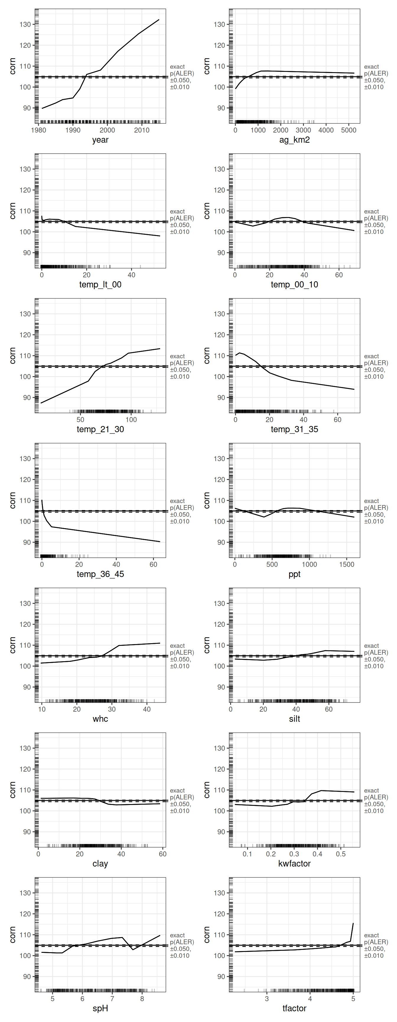
With this view, the plots align cleanly with the ALED rankings: year shows the largest range, followed by the key temperature ranges (especially 21–30°C and 31–35°C). We also interpret these plots with the rug marks in mind. Extreme x-values often have sparse support, so we put most interpretive weight on regions of the predictor where the data are dense and the ALE curve is well supported.
ale_boot_rf_corn |>
  plot() |>  # create ALEPlots object
  subset(list(d2 = TRUE)) |>   # subset only for 2D plots
  print(ncol = 1)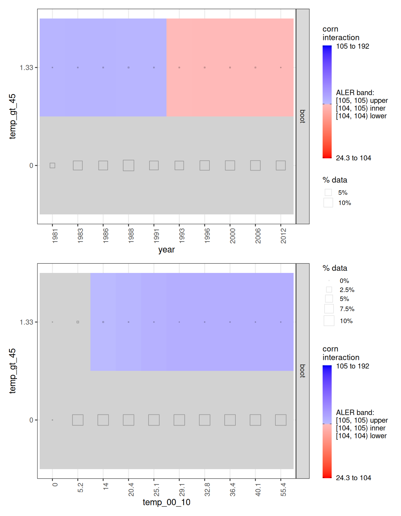
Looking at the interaction plots, the most visible pattern involves year and the number of days with temperatures above 45°C. There appears to be a small regime shift: when there are roughly 1–2 such days, earlier years are associated with higher yield, while later years are associated with lower yield. However, the interaction heatmaps also display the fraction of observations in each cell (the size of the little grey squares within cells). In the “statistically significant” regions, those squares are tiny, often representing less than 1% of the data. In practice, we have very few county-years with days above 45°C, so the interaction, while real and statistically significant, is supported by little data.
A similar caution applies to the interaction between days above 45°C and days in the 0–10°C range. The visual suggests conditional effects, but again the relevant cells are sparsely populated, so we treat these interaction signals as weak and not practically decisive.
8 Conclusion
8.1 Methodological comments
Methodologically, a few lessons stand out.
First, when we constrain all relationships to be linear and do not allow for automatic detection of even small interactions, standard OLS performs only moderately, with SA below 64.6%. The limitation is structural rather than incidental. OLS can only capture what we explicitly specify, and in this setting that restriction costs predictive accuracy.
In contrast, machine learning models such as random forests are well suited to datasets of this size and complexity. Using ranger, we obtain excellent performance with minimal tuning. The model handles nonlinearities and potential interactions automatically, which is precisely what we need here.
Given that performance gap, we focus our interpretation on the random forest model.
A second important methodological result concerns interactions. Although we computed all pairwise ALE interactions, none of them are practically important. The interaction effects are small, and none exceed our threshold of two bushels per acre. This matters. Because interactions do not meaningfully distort the marginal relationships, we can interpret the main effects directly without worrying that strong interaction structure is hiding underneath.
8.2 Key findings
With a dataset of this size, statistical significance is almost guaranteed. Indeed, all effects are statistically significant. That is not the interesting part.
What matters is magnitude. Only eight variables exhibit ALED effects of at least two bushels per acre. These are the effects that clear our threshold for practical importance, and we display their ALE plots accordingly.
# Create variable lists to focus on
vars_aled_2 <- ale_boot_rf_corn |>
  get(stats = 'estimate') |>
  bind_rows() |>
  filter(aled >= 2) |>
  pull(term)

ale_boot_rf_corn |>
  plot() |>  # create ALEPlots object
  subset(vars_aled_2) |>  # subset only for 1D plots
  customize(zoom_y = c(85, 135)) |>   # zoom on the y-axis
  print(ncol = 2)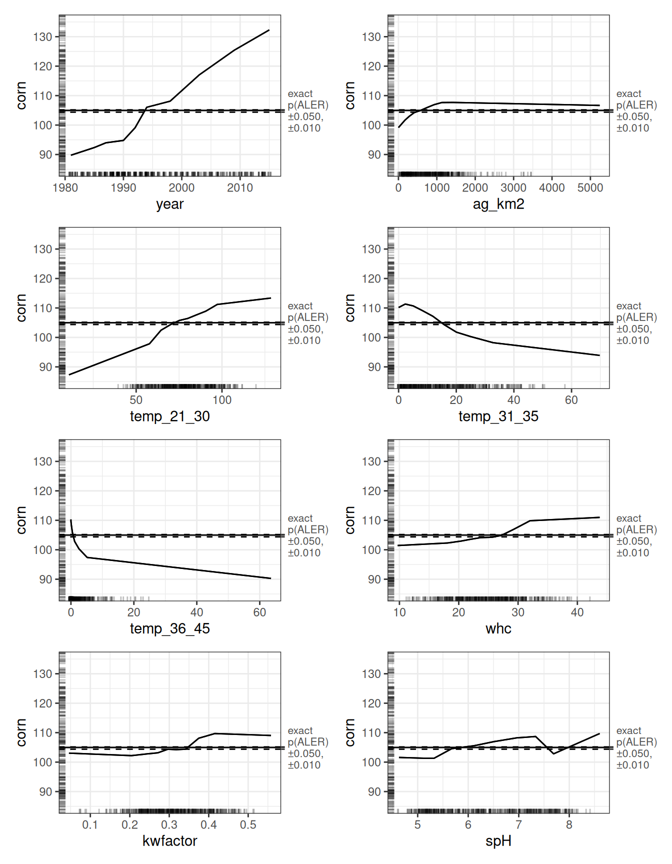
None of the relationships we observe is strictly linear. Still, the overall directions are clear. Corn yield is positively associated with later years, larger agricultural land area in a county (ag_km2), more days in the “ideal” 21–30°C range, and favourable soil characteristics including water holding capacity (whc), kwfactor, and soil pH (spH). In contrast, more days in the 31–35°C or 36–46°C ranges are associated with lower yields.
Although ALE is computationally demanding, it gives us a way to interpret a complex, high-performing machine-learning model while keeping the results on a meaningful scale and attaching statistical confidence where appropriate.
8.3 A note on unsurprising results
Nothing in these main-effect patterns is especially shocking, and that is largely expected. When we analyze a well-known, preassembled dataset, the “headline” relationships have usually been explored already. Where we can realistically expect more novel insights is by merging a rich panel like ACDC (corn, wheat, soybean, cotton, etc.) with other compatible datasets, for example additional county-, state-, or year-indexed measures with very different kinds of data that might not normally be expected to be related to corn, weather, or soil characteristics.
If surprises emerge from such merges, they are likely to come from unexpected interactions rather than from the main effects already embedded in the original sources. That said, interactions also raise their own interpretability challenges, and further development of ALE-based tools for interaction explanation would make those future studies easier to unpack.
9 References
Yun, Seong Do, and Benjamin M. Gramig. 2017. Agro-Climatic Data by County, 1981-2015. Dataset. Purdue University. https://doi.org/10.4231/R72F7KK2.