library(dplyr)  # data manipulation
library(staccuracy)  # performance metrics
library(tictoc)  # performance timing
library(mgcv)  # Generalized Additive Models
library(ranger)  # random forest
library(kableExtra)  # table formatting

# Other packages that must be installed
# Uncomment the following lines as needed.

# # If needed, first install the pak advanced package manager (needed to easily install a package directly from GitHub):
# install.packages('pak')
#
# pak::pak('agridat')  # agricultural datasets
#
# # Accumulated Local Effects: ale package
# # Install the development version of ale for this workshop, which is more recent than the current CRAN version.
# pak::pak('tripartio/ale')
library(ale) # load the ale package only after installing the development versionAnalyzing a Small Rice Yield Dataset with ALE-Based Inference
February 17, 2026
Source:vignettes/ale-gomez-rice.qmd
1 Introduction
We’re working with a tiny, expensive kind of dataset: the sort you get when each data point costs fieldwork, fertilizer, and patience. These rice data come from the International Rice Research Institute (IRRI) and are discussed in Gomez & Gomez (1984).
Our goal is simple: figure out how rice yield responds to nitrogen fertilizer in dry versus wet seasons, and whether the “best” nitrogen level should differ by season.
We’ll analyze the data with three model families:
- OLS regression (classic linear regression).
- Random forest (mostly as a cautionary tale on tiny data).
- Generalized additive model (GAM), which is usually the best fit for “small data + nonlinearity”.
2 Set up R environment
First, let’s set up our R environment. We begin by loading the packages we’ll use. Two quick notes:
- The dataset comes from the {agridat} package (it doesn’t have to be loaded, but it does have to be installed).
- The {ale} package is on CRAN, but for a few features used here we install the current development version from GitHub (the code shows how, via {pak}).
# For speed, these examples use retrieve_rds() to load precreated objects
# from an online repository.
# To run the code yourself, execute the code blocks directly.
serialized_objects_site <- "https://github.com/tripartio/ale/raw/main/download/rice_objects"
3 Data preparation and description
The data come from IRRI in the Philippines. Unfortunately, the book that describes it (Gomez & Gomez, 1984) does not give much context (country/year/site details) beyond this description:
“We give the procedures for analyzing data of experiments over crop seasons using a fertilizer trial with five nitrogen rates tested on rice for two seasons, using a RCB design with three replications” (p. 317).
Preparation is straightforward: we pull gomez.wetdry and convert it to a tibble. We also drop the rep column because it’s not a usable replication ID here. It uses labels like R1/R2/R3, but R1 in one row is not the same experimental block as R1 in another row, so treating it as a factor would invite nonsense, especially with a dataset this small.
We’ll add more commentary later. For now, here’s the full dataset.
rice |> print(n = 50)# A tibble: 30 × 3
season nitrogen yield
<fct> <int> <dbl>
1 dry 0 4.89
2 dry 0 2.58
3 dry 0 4.54
4 dry 60 6.01
5 dry 60 6.62
6 dry 60 5.67
7 dry 90 6.71
8 dry 90 6.69
9 dry 90 6.80
10 dry 120 6.46
11 dry 120 6.68
12 dry 120 6.64
13 dry 150 5.68
14 dry 150 6.87
15 dry 150 5.69
16 wet 0 5.00
17 wet 0 3.50
18 wet 0 5.36
19 wet 60 6.35
20 wet 60 6.32
21 wet 60 6.58
22 wet 90 6.07
23 wet 90 5.97
24 wet 90 5.89
25 wet 120 4.82
26 wet 120 4.02
27 wet 120 5.81
28 wet 150 3.44
29 wet 150 4.05
30 wet 150 3.74After printing the data, we summarize it.
rice |> summary() season nitrogen yield
dry:15 Min. : 0 Min. :2.577
wet:15 1st Qu.: 60 1st Qu.:4.836
Median : 90 Median :5.853
Mean : 84 Mean :5.515
3rd Qu.:120 3rd Qu.:6.551
Max. :150 Max. :6.868
rice$nitrogen |> table()
  0  60  90 120 150
  6   6   6   6   6
Three replications of five nitrogen rates were run in each of the dry and wet seasons, for a total of 30 plots.
-
season(factor): wet or dry season. -
nitrogen(numeric): five nitrogen fertilizer rates applied to each agricultural plot, in kilograms per hectare (kg/ha). -
yield(numeric): rice grain yield, in tonnes per hectare (t/ha), that is, 1,000 kg/ha.
Notably, the outcome variable, rice yield has a mean of 5.5 t/ha and a mean absolute deviation (mad) of 0.982.
4 Model evaluation
Before we train anything, we need to be clear about how we evaluate models. There are two particular principles of our evaluation approach: appropriate metrics for practical alignment and for predictive analysis.
4.1 Metrics for numeric prediction
Classic statistics leans heavily on R² or adjusted R². These measure explained variance. That’s fine as far as it goes, but we want to be more deliberate about our metrics.
Our outcome is a numeric, ratio, continuous variable: yield in t/ha. For tasks like this, the most appropriate metric is usually mean absolute error (MAE).
The problem with MAE–and most metrics–is interpretation. Smaller is better, yes—but how small is good? The standard comparison for MAE is the mean absolute deviation (MAD). For our dataset, the MAD for rice yield is 0.982. Thus, any “good” model should have an MAE smaller than that threshold
To simplify such comparisons, we also use standardized accuracy (staccuracy or SA), from the {staccuracy} package. This rescales performance to a 0–100% range. A value of 100% means perfect prediction. A value of 50% corresponds to predicting the mean every time. So, for MAE staccuracy, 50% is the score of the MAD. Any staccuracy above 50% beats the mean; anything below 50% is worse than simply guessing the mean. We will report both MAE and standardized accuracy.
4.2 Descriptive versus predictive metrics
Descriptive metrics are computed on the full dataset used to train the model. They tell us how well the model reproduces the data it already saw. That is useful, but it is still in-sample performance.
Predictive metrics are more realistic. They train the model on part of the data and evaluate it on data not used in fitting. Common approaches include cross-validation and bootstrapping. Cross-validation is often used for very large datasets or slow models. Bootstrapping works well for small datasets and faster models.
Our dataset is small, so we will use bootstrapping—specifically full-model bootstrapping. We explain the difference between bootstrap approaches in an article on ALE statistics and inference.
Here are the eventual results of our analyses. Note that lower MAE is better, and higher staccuracy (SA) is better. Descriptive metrics usually look better than predictive metrics because they tend to misleadingly overfit the data.
| Model | MAE (t/ha) | SA (%) | MAE (t/ha) | SA (%) |
|---|---|---|---|---|
| OLS | 0.772 | 60.7 | 0.918 | 48.8 |
| Random forest | 0.548 | 72.1 | 0.641 | 64.6 |
| GAM | 0.390 | 80.2 | 0.531 | 70.1 |
With evaluation clarified, we can now move on to the models themselves.
5 OLS regression
5.1 Model training
We start with the most familiar tool in the toolbox: ordinary least squares (OLS) linear regression.
We fit a model using both predictors, season and nitrogen, and we also include their interaction. That means we allow the effect of nitrogen to differ between wet and dry seasons rather than forcing one shared slope.
After fitting the model, we print the summary to inspect coefficients, standard errors, and overall fit.
lm_rice <- lm(
  yield ~ season + nitrogen + season:nitrogen,
  data = rice
)
sa_lm_rice  <- sa_wmae_mad(rice$yield, predict(lm_rice))  # 0.60739
mae_lm_rice <- mae(rice$yield, predict(lm_rice))  # 0.7719829
summary(lm_rice)
Call:
lm(formula = yield ~ season + nitrogen + season:nitrogen, data = rice)

Residuals:
    Min      1Q  Median      3Q     Max
-2.1507 -0.6644  0.1648  0.8069  1.3039

Coefficients:
                    Estimate Std. Error t value Pr(>|t|)
(Intercept)         4.664225   0.497790   9.370 8.08e-10 ***
seasonwet           0.989486   0.703982   1.406  0.17169
nitrogen            0.014739   0.005049   2.919  0.00716 **
seasonwet:nitrogen -0.020999   0.007140  -2.941  0.00679 **
---
Signif. codes:  0 '***' 0.001 '**' 0.01 '*' 0.05 '.' 0.1 ' ' 1

Residual standard error: 1.009 on 26 degrees of freedom
Multiple R-squared:  0.3576,    Adjusted R-squared:  0.2835
F-statistic: 4.824 on 3 and 26 DF,  p-value: 0.008423
Before interpreting the OLS coefficients, we check whether the model is doing anything useful. The adjusted R2 is 0.284 (1.0 would be perfect), which is… not inspiring, and it’s also not a metric with a clean “good/bad” cutoff.
In the coefficient table, the season effect is not statistically significant. Nitrogen is statistically significant (p ⩽ 0.05), but the estimated slope (0.015) is tiny, and the season × nitrogen interaction is also significant but tiny at -0.021.
Using our preferred metrics, the OLS model has a descriptive MAE of 0.772 t/ha and standardized accuracy of 60.7%. That staccuracy is better than coin-flip territory, but these are still descriptive metrics and can look deceptively good on small data.
So we move to ALE to understand what the model is actually implying.
5.2 ALE analysis
We start with a single ALE explanation (fast here because we only have two predictors and one interaction). We’ll focus on ALED (ALE deviation) as our main effect-size summary. We explain this and other ALE statistics in detail in another article.
# Single ALE description
ale_lm_rice <- ALE(
  lm_rice,
  x_cols = list(d1 = TRUE, d2 = TRUE),
  data = rice,
  # p_values = pd_lm_rice,
  parallel = 0
)

summary(ale_lm_rice)
# A tibble: 3 × 7
term aled aler_min aler_max naled naler_min naler_max
<chr> <dbl> <dbl> <dbl> <dbl> <dbl> <dbl>
1 season 0.387 -0.387 0.387 13.3 -13.3 13.3
2 nitrogen 0.153 -0.318 0.318 9.33 -13.3 13.3
3 season:nitrogen 0.391 -1.04 0.614 14.3 -26.7 23.3# A tibble: 6 × 7
statistic term estimate conf.low mean median conf.high
<ord> <chr> <dbl> <dbl> <dbl> <dbl> <dbl>
1 aled season 0.387 0.387 0.387 0.387 0.387
2 aled nitrogen 0.153 0.153 0.153 0.153 0.153
3 aled season:nitrogen 0.391 0.391 0.391 0.391 0.391
4 naled season 13.3 13.3 13.3 13.3 13.3
5 naled nitrogen 9.33 9.33 9.33 9.33 9.33
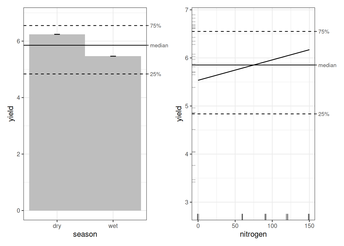
6 naled season:nitrogen 14.3 14.3 14.3 14.3 14.3 # A tibble: 0 × 0From the ALE summary, the season ALED effect is about 0.387 t/ha (≈ 387 kg/ha) and that for nitrogen is about 153 kg/ha. The season × nitrogen interaction ALED is about 391 kg/ha. However, note that without bootstrapping, these results shouldn’t be considered reliable.
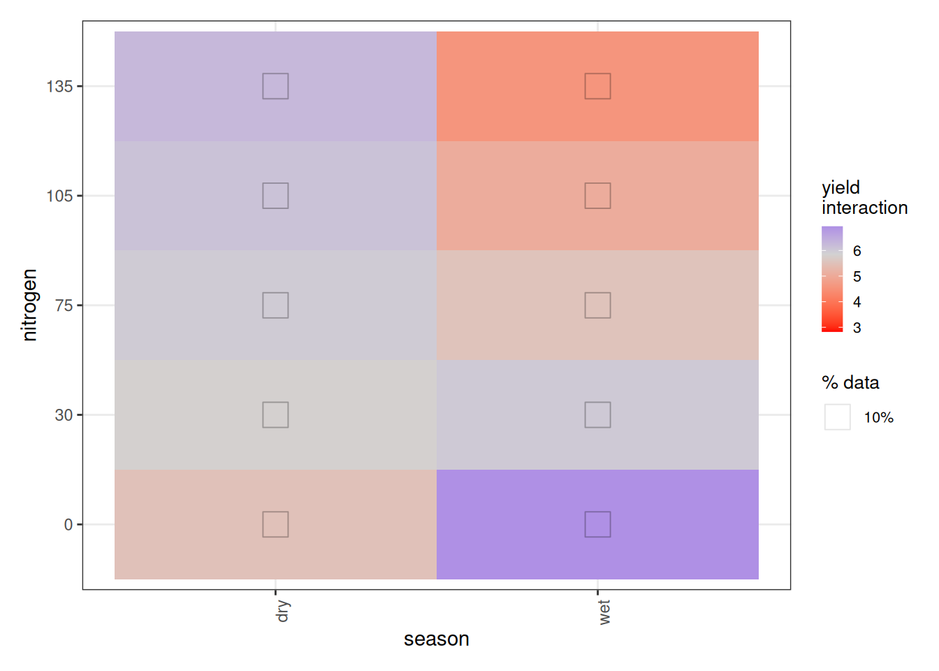
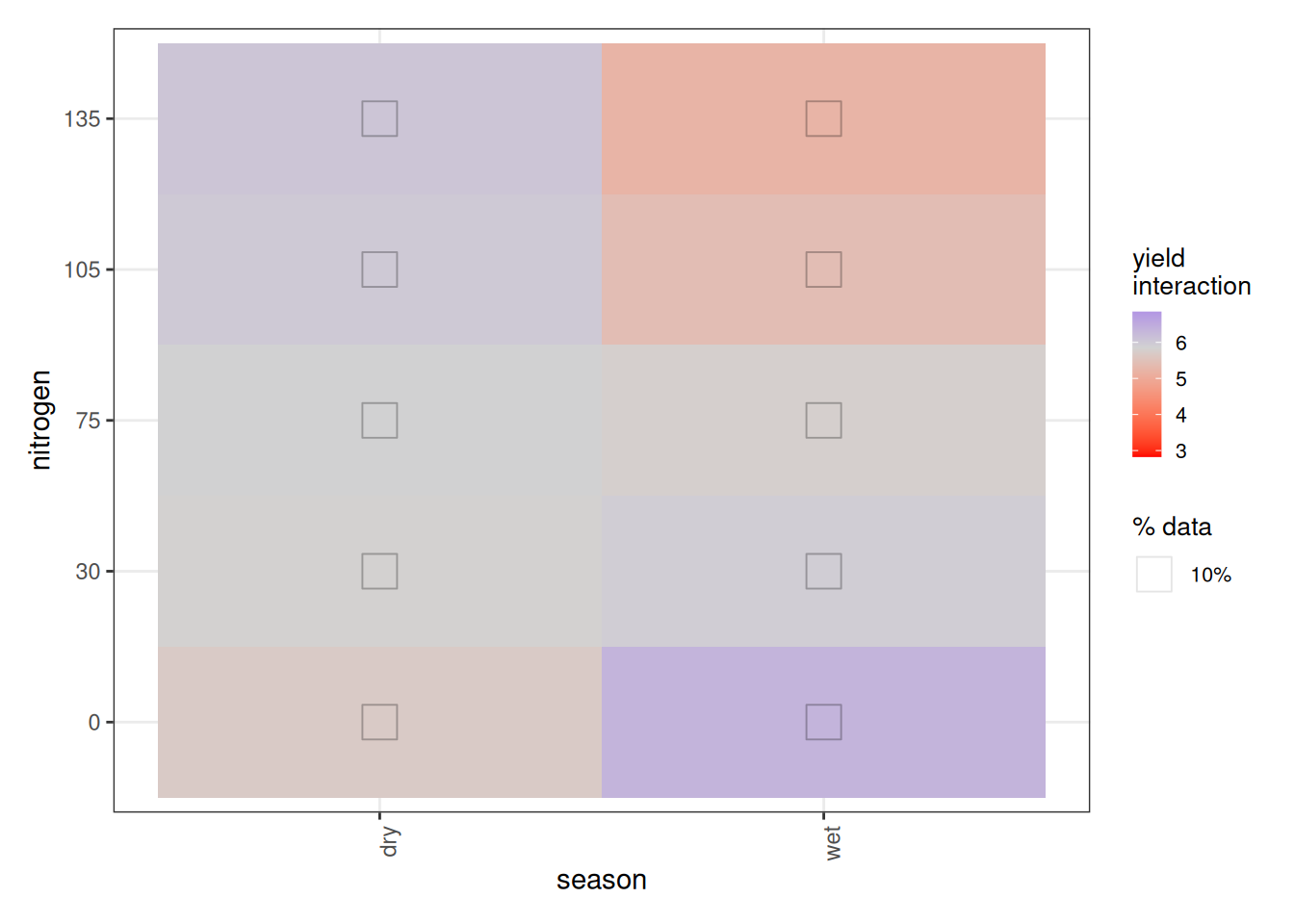
Next we look at the ALE plots. With only three terms, we’ll inspect them all (in bigger studies, we’d be pickier).
For the ALE analysis of the OLS model, we begin with the statistics before turning to the plots. Since ALE is run only once here, relying on p-values alone would not be very informative. We obtain ALED estimates, which we have already defined elsewhere.
Looking at the plots again, the pattern is consistent: dry-season yield appears higher than wet-season yield, and the OLS model implies that more nitrogen increases yield overall. The interaction suggests that nitrogen may reduce yield in the wet season, but we’ll hold off on interpreting the interaction plots until we come to the GAM further down.
However, statistical results (ALE or otherwise) are generally not reliable until we bootstrap them.Because our dataset is tiny and the models train quickly, we use full model bootstrapping. There are two ways to bootstrap ALE. The faster approach resamples only the ALE calculation data without retraining the model. That approach is appropriate for very large datasets and very slow models that have already been validated by cross-validation.
That is not our situation. We have a small dataset and fast models. So we must retrain the entire model for each bootstrap iteration. By default, we use 100 bootstrap iterations. For publication, we could increase that number, but for analysis, 100 iterations are typically sufficient and lead to the same conclusions. ALE itself is relatively stable compared to some other interpretability methods.
Before bootstrapping, let’s first generate an ALE p-value distribution. This is the slowest step in ALE analysis because it relies on simulation rather than parametric assumptions. Whenever procedures are slow in this demonstration, the code blocks are commented out and presaved objects are loaded instead, so the document runs quickly.
We can then use the p-value distribution for the full-model bootstrapping procedure from the {ale} package, to create a ModelBoot object. We explicitly request ALE for season, nitrogen, and the season × nitrogen interaction. Only after this full bootstrap process do the ALE results become reliable
# SLOW: uncomment to run yourself; load the saved object for rapid execution

# # p-value distribution
# # Default 1000 iterations for exact p-values
# tic()
# pd_lm_rice <- ALEpDist(lm_rice, rice, parallel = 0)
# toc()  # 542.13 sec elapsed
# # saveRDS(pd_lm_rice, file.choose())

pd_lm_rice <- serialized_objects_site |>
  file.path("pd_lm_rice.rds") |>
  url() |>
  readRDS()


# SLOW: uncomment to run yourself; load the saved object for rapid execution

# # Full-model bootstrapped ALE explanation
# # Default 100 bootstrap iterations
# tic()
# mb_lm_rice <- ModelBoot(
#   lm_rice, rice,
#   ale_options = list(x_cols = c('season', 'nitrogen', 'season:nitrogen')),
#   ale_p = pd_lm_rice,
#   parallel = 0
# )
# toc()  # 113.02 sec elapsed
# # saveRDS(mb_lm_rice, file.choose())

mb_lm_rice <- serialized_objects_site |>
  file.path("mb_lm_rice.rds") |>
  url() |>
  readRDS()
summary(mb_lm_rice) # boot_valid SA 48.8%: MAE 0.918# A tibble: 12 × 7
name boot_valid conf.low median mean conf.high sd
<chr> <dbl> <dbl> <dbl> <dbl> <dbl> <dbl>
1 r.squared NA 0.193 0.444 0.449 0.715 0.134
2 adj.r.squared NA 0.100 0.380 0.385 0.682 0.150
3 sigma NA 0.621 0.907 0.907 1.13 0.137
4 statistic NA 2.08 6.92 8.25 21.8 5.34
5 p.value NA 0 0.0014 0.0129 0.130 0.0323
6 df NA 3 3 3 3 0
7 df.residual NA 26 26 26 26 0
8 nobs NA 30 30 30 30 0
9 mae 0.918 0.634 NA NA 1.45 0.232
10 sa_mae 0.488 -0.0793 NA NA 0.649 0.191
11 rmse 1.14 0.770 NA NA 2.12 0.354
12 sa_rmse 0.498 0.0366 NA NA 0.652 0.176 # A tibble: 4 × 6
term conf.low median mean conf.high std.error
<chr> <dbl> <dbl> <dbl> <dbl> <dbl>
1 (Intercept) 3.56 4.68 4.71 6.34 0.697
2 seasonwet -0.550 1.16 1.27 4.18 1.20
3 nitrogen 0.0005 0.0149 0.0148 0.0273 0.007
4 seasonwet:nitrogen -0.0483 -0.0236 -0.0236 -0.0063 0.0114# A tibble: 3 × 7
term aled aler_min aler_max naled naler_min naler_max
<fct> <dbl> <dbl> <dbl> <dbl> <dbl> <dbl>
1 season 0.405 -0.416 0.421 14.9 -13.4 17.2
2 nitrogen 0.200 -0.391 0.463 8.69 -13.3 21.5
3 season:nitrogen 0.409 -1.06 0.793 15.0 -24.2 31.3# A tibble: 6 × 8
statistic term estimate p.value conf.low median mean conf.high
<ord> <fct> <dbl> <dbl> <dbl> <dbl> <dbl> <dbl>
1 aled season 0.405 0.006 0.0483 0.445 0.405 0.860
2 aled nitrogen 0.200 0.212 0.0245 0.184 0.200 0.463
3 aled season:nitrogen 0.409 0.005 0.113 0.392 0.409 0.789
4 naled season 14.9 0.053 0.581 14.9 14.9 33.1
5 naled nitrogen 8.69 0.235 0 8.33 8.69 20.7
6 naled season:nitrogen 15.0 0.049 1.32 14.6 15.0 28.6 # A tibble: 0 × 0Bootstrapping gives us predictive metrics based on bootstrap validation on 100 hold-out samples. The OLS model has a predictive MAE of 0.918 t/ha and standardized accuracy of 48.8%. Any staccuracy less than 50% counts as a “bad” model–it’s worse than simply predicting the mean every time. So, our OLS model is pretty much useless. At least, we’ve learnt that we can’t trust it.
This is reinforced by the complete absence of statistically significant confidence regions–ALE-based inference is telling us that we can’t trust anything this model says.
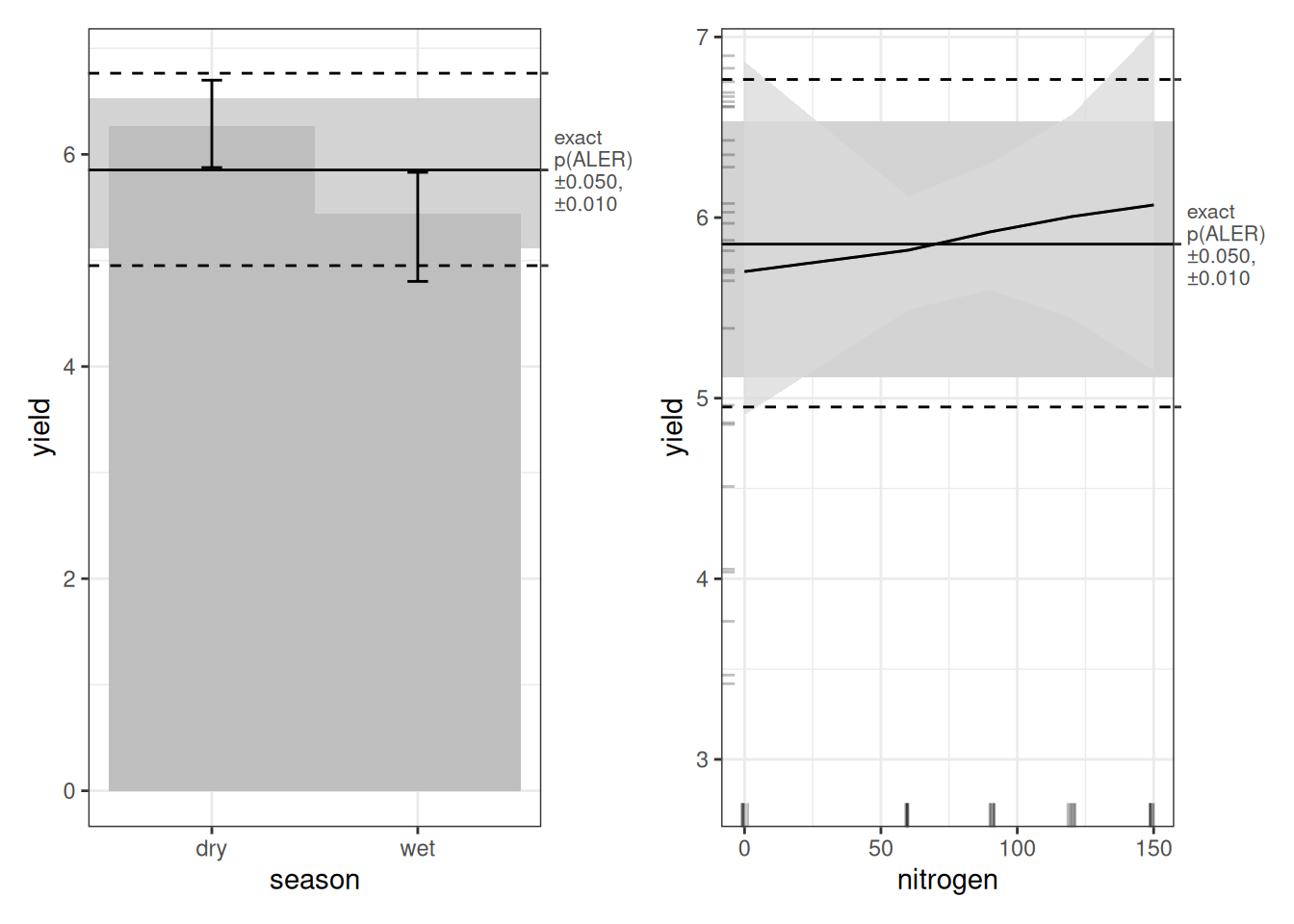
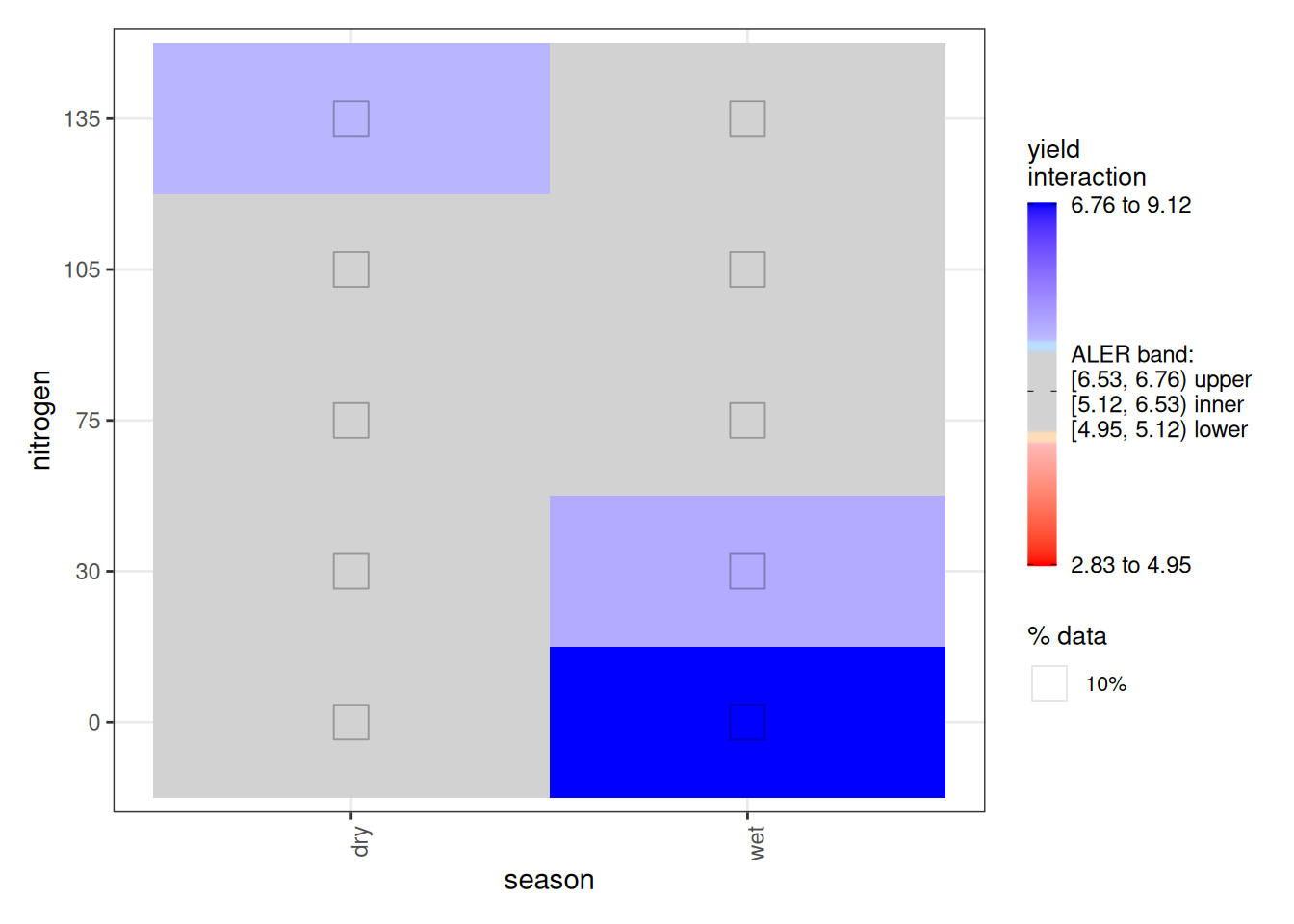
Plotting the bootstrapped ALE reinforces our scepticism: all results fall within the middle grey ALER band, which indicates where random results live. Although the 2D interaction plot has some regions outside the ALER band, the statistics above indicate that the bootstrapped ranges nonetheless overlap the ALER band, which is not shown in this plot.
6 Random forest
Next we analyze the data using a random forest model. Let’s be honest upfront: random forest is not well suited for a dataset this small. We include it anyway for demonstration purposes—to show that machine learning is not automatically the best solution. Model choice should match the data, not the hype.
We use {ranger}, a fast and easy-to-use random forest implementation in R. Tree-based models come in three main varieties:
- Single decision trees.
- Random forests build many decision trees on bootstrapped samples and average them with bootstrap aggregation (bagging).
- Gradient boosted trees also builds multiple trees, but sequentially, each correcting the previous one, though a procedure called boosting.
Gradient boosted trees often perform extremely well, but here we use {ranger} for random forests because it is fast, simple, and performs well with default settings.
6.1 Model training
Because random forest is stochastic, we set a random seed. Otherwise, each run would produce slightly different results. Beyond that, we use the default settings.
# Precise performance metrics vary slightly for a random forest
rf_rice <- ranger(
  yield ~ .,
  data = rice,
  seed = 1  # ensure that the same random forest is generated each time
)
sa_rf_rice  <- sa_wmae_mad(rice$yield, predict(rf_rice, rice)$predictions)  # 0.7222866
mae_rf_rice <- mae(rice$yield, predict(rf_rice, rice)$predictions)  # 0.5429936
rf_rice
Ranger result
Call:
ranger(yield ~ ., data = rice, seed = 1)
Type: Regression
Number of trees: 500
Sample size: 30
Number of independent variables: 2
Mtry: 1
Target node size: 5
Variable importance mode: none
Splitrule: variance
OOB prediction error (MSE): 0.7410144
R squared (OOB): 0.4787994 The random forest has a descriptive MAE of 0.548 t/ha and standardized accuracy of 72.1%. Descriptively, this looks much better than OLS. But descriptive performance is the easy part.
6.2 ALE analysis
The {ale} package automatically recognizes the {ranger} package, so using default settings, it easily creates an ALE explanation.
# Single ALE description
ale_rf_rice <- ALE(
  rf_rice,
  x_cols = list(d1 = TRUE, d2 = TRUE),
  data = rice,
  # p_values = pd_rf_rice,
  parallel = 0
)

summary(ale_rf_rice)
# A tibble: 3 × 7
term aled aler_min aler_max naled naler_min naler_max
<chr> <dbl> <dbl> <dbl> <dbl> <dbl> <dbl>
1 season 0.358 -0.358 0.358 13.3 -13.3 13.3
2 nitrogen 0.255 -0.848 0.409 11.3 -16.7 13.3
3 season:nitrogen 0.185 -0.543 0.290 7.67 -16.7 13.3# A tibble: 6 × 7
statistic term estimate conf.low mean median conf.high
<ord> <chr> <dbl> <dbl> <dbl> <dbl> <dbl>
1 aled season 0.358 0.358 0.358 0.358 0.358
2 aled nitrogen 0.255 0.255 0.255 0.255 0.255
3 aled season:nitrogen 0.185 0.185 0.185 0.185 0.185
4 naled season 13.3 13.3 13.3 13.3 13.3
5 naled nitrogen 11.3 11.3 11.3 11.3 11.3
6 naled season:nitrogen 7.67 7.67 7.67 7.67 7.67 # A tibble: 0 × 0
In the random forest ALE plots, the season effect is very similar to that of ordinary least squares, but the nitrogen fertilizer effect is quite different. Here, nitrogen shows an inverted-U pattern (peaking around 60–90 kg/ha), and the interaction again suggests different nitrogen behaviour across seasons. Still, we shouldn’t get too excited until we check predictive stability.
# SLOW: uncomment to run yourself; load the saved object for rapid execution

# # p-value distribution
# # Default 1000 iterations for exact p-values
# tic()
# pd_rf_rice <- ALEpDist(
#   rf_rice, rice,
#   parallel = 0
# )
# toc()  # 560.64 sec elapsed
# # saveRDS(pd_rf_rice, file.choose())

pd_rf_rice <- serialized_objects_site |>
  file.path("pd_rf_rice.rds") |>
  url() |>
  readRDS()


# SLOW: uncomment to run yourself; load the saved object for rapid execution

# # Full-model bootstrapped ALE explanation
# # Default 100 bootstrap iterations
# tic()
# mb_rf_rice <- ModelBoot(
#   rf_rice, rice,
#   ale_options = list(x_cols = c('season', 'nitrogen', 'season:nitrogen')),
#   ale_p = pd_rf_rice,
#   parallel = 0
# )
# toc()  # 70.89 sec elapsed
# # saveRDS(mb_rf_rice, file.choose())

mb_rf_rice <- serialized_objects_site |>
  file.path("mb_rf_rice.rds") |>
  url() |>
  readRDS()
summary(mb_rf_rice) # boot_valid SA 64.6%; MAE 0.6400844# A tibble: 4 × 7
name boot_valid conf.low median mean conf.high sd
<chr> <dbl> <dbl> <dbl> <dbl> <dbl> <dbl>
1 mae 0.641 0.421 NA NA 0.950 0.141
2 sa_mae 0.646 0.363 NA NA 0.744 0.108
3 rmse 0.807 0.520 NA NA 1.27 0.209
4 sa_rmse 0.647 0.404 NA NA 0.735 0.0804# A tibble: 3 × 7
term aled aler_min aler_max naled naler_min naler_max
<fct> <dbl> <dbl> <dbl> <dbl> <dbl> <dbl>
1 season 0.339 -0.349 0.350 13.6 -13.2 14.7
2 nitrogen 0.256 -0.868 0.433 11.6 -21.8 18.5
3 season:nitrogen 0.188 -0.523 0.331 8.17 -17.0 14.0# A tibble: 6 × 8
statistic term estimate p.value conf.low median mean conf.high
<ord> <fct> <dbl> <dbl> <dbl> <dbl> <dbl> <dbl>
1 aled season 0.339 0.008 0.0813 0.352 0.339 0.580
2 aled nitrogen 0.256 0.054 0.144 0.240 0.256 0.400
3 aled season:nitrogen 0.188 0.205 0.0904 0.180 0.188 0.301
4 naled season 13.6 0.059 1.59 13.8 13.6 24.7
5 naled nitrogen 11.6 0.225 2.88 11.1 11.6 20.7
6 naled season:nitrogen 8.17 0.835 2.17 7.67 8.17 15.2 # A tibble: 0 × 0Once we bootstrap, the performance is less impressive than with purely descriptive metrics. The random forest has a predictive MAE of 0.641 t/ha and standardized accuracy of 64.6%. That said, the staccuracy of above 50% indicates that this is at least a decent model. However, we will see that we can do better, as random forests don’t shine best on small datasets like this.
We’ll hold off deeper interpretation of the random forest plots and focus our main interpretation on the GAM.
7 GAM
Now we move to generalized additive models (GAMs). A GAM sits within the broader generalized linear model (GLM) family, but unlike standard linear regression (OLS), it allows nonlinear relationships. Instead of forcing straight lines, it lets the data determine the shape of the relationship. When properly configured, GAMs work especially well on small datasets like ours. They offer flexibility without giving up structure.
7.1 Model training
Appropriately configuring GAMs is as much an art as a science, and so we won’t get into how we arrived at the specific configuration that we use here. However, its key structure is straightforward. We model yield as a function of season, and we include nitrogen through its interaction with season. That means nitrogen is not entered as a simple main effect; instead, its relationship with yield is allowed to differ by season. In this way, nitrogen is fully incorporated into the model. We use the {mgcv} package for the GAM.
gam_rice <- gam(
  yield ~ season + ti(nitrogen, by = season, bs = "ps"),
  data = rice,
  # REML is recommended for more accurate estimation, though slightly slower
  method = 'REML'
)
# workaround a pgkdown bug (probably temporary)
gam_preds <- predict(gam_rice) |> as.numeric()
sa_gam_rice  <- sa_wmae_mad(rice$yield, gam_preds)  # 0.8015714
mae_gam_rice <- mae(rice$yield, gam_preds)  # 0.3898126
summary(gam_rice)
Family: gaussian
Link function: identity

Formula:
yield ~ season + ti(nitrogen, by = season, bs = "ps")

Parametric coefficients:
            Estimate Std. Error t value Pr(>|t|)
(Intercept)   5.9023     0.1556  37.931   <2e-16 ***
seasonwet    -0.7744     0.2201  -3.519   0.0018 **
---
Signif. codes:  0 '***' 0.001 '**' 0.01 '*' 0.05 '.' 0.1 ' ' 1

Approximate significance of smooth terms:
                         edf Ref.df     F  p-value
ti(nitrogen):seasondry 2.141  2.387 16.01 2.07e-05 ***
ti(nitrogen):seasonwet 2.346  2.636 14.55 4.57e-05 ***
---
Signif. codes:  0 '***' 0.001 '**' 0.01 '*' 0.05 '.' 0.1 ' ' 1

R-sq.(adj) =  0.745   Deviance explained = 79.3%
-REML = 30.862  Scale est. = 0.36319   n = 30
We won’t over-interpret the GAM coefficients; the more useful story here comes from performance and the ALE surfaces.
The adjusted R-squared is 0.745, but we don’t compare that number directly to OLS or random forest, because different model classes compute “R-squared” in different ways. MAE and standardized accuracy are comparable across models, though.
Using our preferred, comparable metrics, the GAM has a descriptive MAE of 0.39 t/ha and standardized accuracy of 80.2%. So far, this is our best descriptive performance. We emphasize, though, that only prescriptive metrics are reliable.
In the parametric part of the GAM summary, season shows a negative shift going from dry to wet (lower yield in wet), which is statistically significant. Nitrogen is included via its season-specific smooth interaction, so its effect isn’t summarized as a single tidy coefficient.
There is no interpretable coefficient for the interaction between season and nitrogen. What we see instead is the estimated degrees of freedom (EDF), which tell us to what extent the interaction is nonlinear. The statistically significant EDFs confirm nonlinearity, but do not describe the direction or shape of the effect. GAM requires plots for that interpretive step.
This is exactly why we turn to ALE. ALE incorporates the full structure of the model and allows us to visualize and quantify the effect of nitrogen even though it was not specified as a simple parametric term.
7.2 Single ALE on entire dataset
Next, we use ALE to examine the shape of the fitted relationships and give us model-agnostic statistics.
# Single ALE description
ale_gam_rice <- ALE(
  gam_rice,
  x_cols = list(d1 = TRUE, d2 = TRUE),
  data = rice,
  # p_values = pd_gam_rice,
  parallel = 0
)

summary(ale_gam_rice)
# A tibble: 3 × 7
term aled aler_min aler_max naled naler_min naler_max
<chr> <dbl> <dbl> <dbl> <dbl> <dbl> <dbl>
1 season 0.387 -0.387 0.387 13.3 -13.3 13.3
2 nitrogen 0.400 -1.28 0.648 15.3 -26.7 23.3
3 season:nitrogen 0.408 -1.16 0.636 15 -26.7 23.3# A tibble: 6 × 7
statistic term estimate conf.low mean median conf.high
<ord> <chr> <dbl> <dbl> <dbl> <dbl> <dbl>
1 aled season 0.387 0.387 0.387 0.387 0.387
2 aled nitrogen 0.400 0.400 0.400 0.400 0.400
3 aled season:nitrogen 0.408 0.408 0.408 0.408 0.408
4 naled season 13.3 13.3 13.3 13.3 13.3
5 naled nitrogen 15.3 15.3 15.3 15.3 15.3
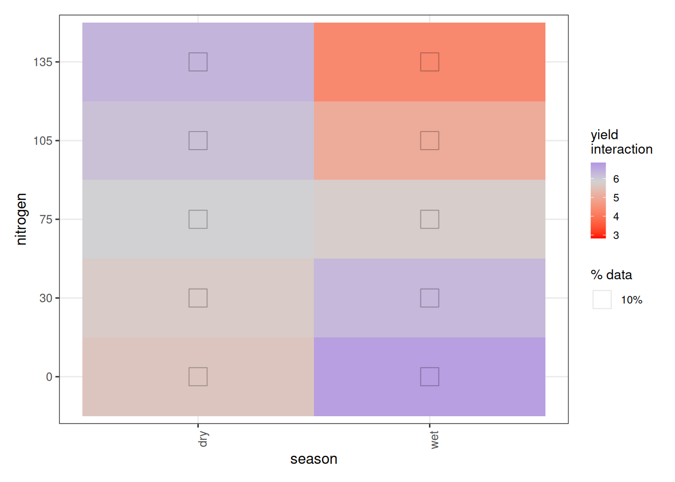
6 naled season:nitrogen 15 15 15 15 15 # A tibble: 0 × 0In the ALE summary, the GAM shows larger ALED effects (roughly 400 kg/ha scale) for season, nitrogen, and their interaction than the earlier models. We’ll interpret these more carefully once we look at the plots.
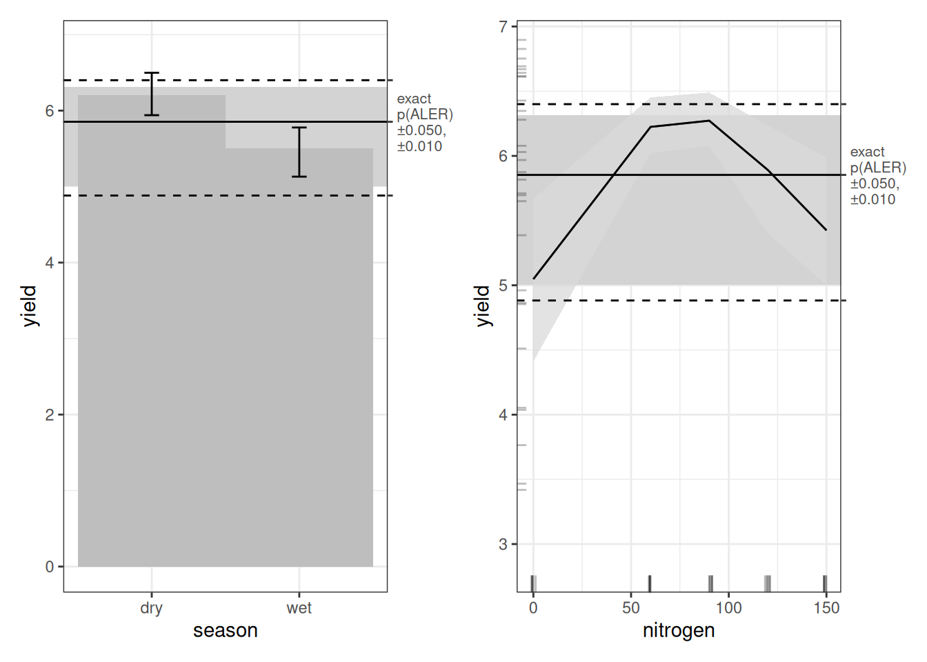
The season main-effect plot is identical to what we saw under OLS, as can be expected, since GAM treats simple factor variables the same way OLS does.
Nitrogen is a different story. Under OLS, the effect looked roughly linear and increasing. Under the GAM, we see something more realistic. Yield is lowest at zero nitrogen, rises sharply, peaks around 60–75 kg/ha, and then declines at higher levels. At 120 and 150 kg/ha, yield drops relative to the peak. In other words, we see an inverted U-shape. This is consistent with what we observed in the {ranger} model.
Now we turn to the nitrogen × season interaction. At first glance, the plot appears to suggest that less fertilizer gives better yields in the wet season, while more fertilizer benefits the dry season. That interpretation would be misleading.
In fact, ALE has a structural quirk when interactions are present. With no interactions, 1D ALE plots reflect intuitive main effects. But once interactions exist:
- 1D ALE (main effects) represent the total effect of that variable, including all its interaction effects.
- 2D ALE interaction plots represent only the additional interaction component, after subtracting the composite main effects.
So in our case:
- The season ALE plot reflects the total season effect, including its interaction with nitrogen.
- The nitrogen ALE plot reflects the total nitrogen effect, including its interaction with season.
- The season × nitrogen plot shows only the extra interaction effect beyond those two main effects.
This means the interaction surface is not saying that more nitrogen reduces yield in the wet season overall. Instead, given the inverted U-shape, it tells us that the dry season tolerates higher nitrogen better, while the wet season declines more sharply past the peak. The extremes of very low or very high nitrogen behave differently across seasons once the shared nonlinear pattern is removed.
Admittedly, this decomposition is not especially intuitive. It is a known limitation of the ALE formulation and an area where interpretation requires care.
7.3 ALE on bootstrapped models
So far, these are preliminary patterns. To assess reliability, we now generate a p-value distribution and perform full model bootstrapping of the GAM.
# SLOW: uncomment to run yourself; load the saved object for rapid execution

# # p-value distribution
# # Default 1000 iterations for exact p-values
# tic()
# pd_gam_rice <- ALEpDist(gam_rice, rice, parallel = 0)
# toc()  # 612.22 sec elapsed
# # saveRDS(pd_gam_rice, file.choose())

pd_gam_rice <- serialized_objects_site |>
  file.path("pd_gam_rice.rds") |>
  url() |>
  readRDS()


# SLOW: uncomment to run yourself; load the saved object for rapid execution

# # Full-model bootstrapped ALE explanation
# # Default 100 bootstrap iterations
# tic()
# mb_gam_rice <- ModelBoot(
#   gam_rice, rice,
#   ale_options = list(x_cols = c('season', 'nitrogen', 'season:nitrogen')),
#   ale_p = pd_gam_rice,
#   parallel = 0
# )
# toc()  # 83.5 sec elapsed
# # saveRDS(mb_gam_rice, file.choose())

mb_gam_rice <- serialized_objects_site |>
  file.path("mb_gam_rice.rds") |>
  url() |>
  readRDS()
summary(mb_gam_rice) # boot_valid SA 70.0%; MAE 0.531# A tibble: 9 × 7
name boot_valid conf.low median mean conf.high sd
<chr> <dbl> <dbl> <dbl> <dbl> <dbl> <dbl>
1 df NA 5.63 6.57 6.64 7.50 0.478
2 df.residual NA 22.5 23.4 23.4 24.4 0.478
3 nobs NA 30 30 30 30 0
4 adj.r.squared NA 0.691 0.817 0.817 0.953 0.0684
5 npar NA 10 10 10 10 0
6 mae 0.531 0.311 NA NA 1.21 0.216
7 sa_mae 0.700 0.295 NA NA 0.835 0.159
8 rmse 0.732 0.427 NA NA 1.88 0.324
9 sa_rmse 0.673 0.12 NA NA 0.823 0.171 # A tibble: 2 × 6
term conf.low median mean conf.high std.error
<chr> <dbl> <dbl> <dbl> <dbl> <dbl>
1 ti(nitrogen):seasondry 1.70 2.19 2.20 2.73 0.261
2 ti(nitrogen):seasonwet 1.11 2.45 2.44 3.20 0.408# A tibble: 3 × 7
term aled aler_min aler_max naled naler_min naler_max
<fct> <dbl> <dbl> <dbl> <dbl> <dbl> <dbl>
1 season 0.394 -0.406 0.409 14.7 -13.5 16.8
2 nitrogen 0.389 -1.31 0.687 15.6 -28.1 29.7
3 season:nitrogen 0.418 -1.15 0.769 15.7 -25.4 30.5# A tibble: 6 × 8
statistic term estimate p.value conf.low median mean conf.high
<ord> <fct> <dbl> <dbl> <dbl> <dbl> <dbl> <dbl>
1 aled season 0.394 0 0.0529 0.404 0.394 0.708
2 aled nitrogen 0.389 0 0.207 0.382 0.389 0.604
3 aled season:nitrogen 0.418 0 0.236 0.404 0.418 0.678
4 naled season 14.7 0.006 0.581 14.8 14.7 29.9
5 naled nitrogen 15.6 0.003 5.21 14.9 15.6 26.8
6 naled season:nitrogen 15.7 0.003 6.76 15.2 15.7 26.4 # A tibble: 6 × 8
term1 x1 term2 x2 aler_band n pct y
<chr> <chr> <chr> <chr> <ord> <int> <dbl> <dbl>
1 season dry nitrogen [0,60] overlap 6 20 5.61
2 season wet nitrogen [0,60] overlap 6 20 6.59
3 season dry nitrogen (60,120] overlap 6 20 6.04
4 season wet nitrogen (60,120] overlap 6 20 5.33
5 season dry nitrogen (120,150] overlap 3 10 6.35
6 season wet nitrogen (120,150] below 3 10 4.44The GAM has a predictive MAE of 0.531 t/ha and standardized accuracy of 70.1%. While this represents a drop of 10% staccuracy from the descriptive to the predictive model, as can be expected with such a small dataset, this nonetheless represents our most accurate model. Thus, we will interpret these bootstrapped results in earnest, since it’s the best that we have.
In the bootstrapped ALE results, all three relationships (season and nitrogen main effects and the season × nitrogen interaction effect) come out highly significant by p-values (p < 0.001), with effect sizes around 400 kg/ha.
Notably, compared to the OLS and random forest results, our more accurate GAM is the only model to produce statistically significant confident regions, which it does for the season × nitrogen interaction. We can better interpret the implications of this when examining the bootstrapped plots.
One caution: ALE “main effects” include interaction contributions by design. The season main effect includes the season–nitrogen interaction (excluding nitrogen-only effects), and the nitrogen main effect includes the interaction (excluding season-only effects). The 2D interaction surface is the part beyond the two main effects. That’s slightly awkward, but it’s the standard ALE definition, so we must carefully interpret results accordingly.
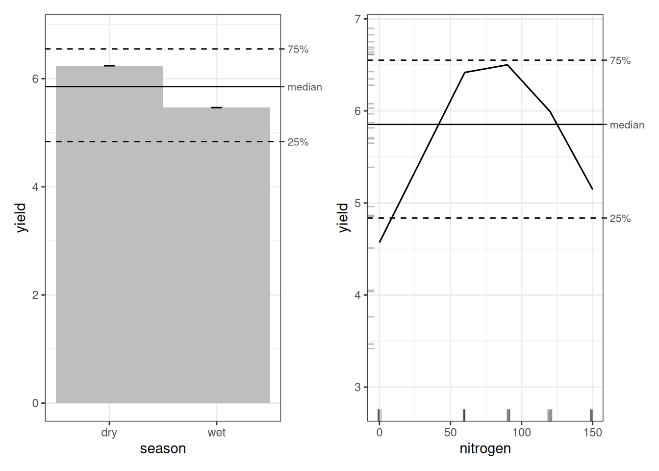
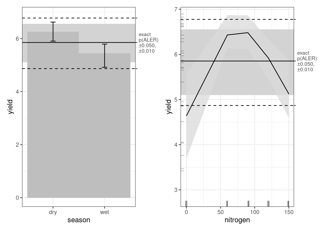
Let’s look first at the main-effect plots. As with every model, dry-season yield appears higher than wet-season yield. And as with the random forest model, we see the inverted U-shape for nitrogen. However, in both cases, the ALER band is very wide. That tells us uncertainty is high. The ALER band represents the range of variation that could plausibly be random. In both main effects, the bootstrap confidence regions do not clearly exceed that band. In other words, even though the curves look different, the differences are not beyond what random fluctuation could produce. With only 30 observations, this is not surprising. It is not necessarily that the relationships do not exist; it is more likely that they would be borne out if we had more replications of this experiment.
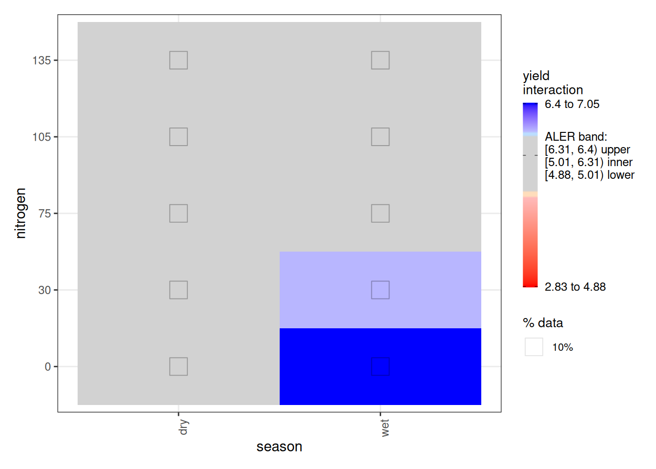
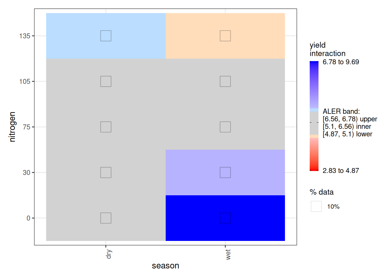
Turning to the interaction plot, most of the surface overlaps the ALER band, which is why much of it appears grey. At the extremes, however, there are strong indications of structure. In the dry season, the highest nitrogen level (150 kg/ha) slightly exceeds the ALER band, suggesting stronger response at high nitrogen. In contrast, in the wet season, the lowest yields occur at the highest nitrogen levels, and the strongest yields occur at lower nitrogen–these boundaries exceed the ALER band of randomness.
The ALE statistics confirm that only the interaction effect meets the significance criterion under ALE-based inference, based on at least 10% of the surface falling outside the two-dimensional ALER band. The main effects remain within the band and therefore are not statistically significant.
8 Discussion
8.1 Comparison with Gomez and Gomez (1984)
In Section 8.1.1, Gomez and Gomez (1984) analyze this dataset using a randomized complete block design and a combined ANOVA over seasons. They conclude that nitrogen significantly affects yield. The season × nitrogen interaction is highly significant. The overall nitrogen response is quadratic. And the seasonal difference lies mainly in the linear component of that quadratic curve. In practical terms, they conclude that yield increases more sharply with nitrogen in the dry season and compute separate yield-maximizing and profit-maximizing nitrogen rates for dry and wet seasons. They explicitly recommend different nitrogen applications by season.
We should note that their modelling approach is not directly comparable to our initial OLS specification. They imposed a quadratic structure on nitrogen. That requires prior knowledge of the expected response shape. We avoided that assumption by using a GAM, which detects nonlinearities automatically and defaults to linear relationships when appropriate. The tradeoff is that flexibility reduces classical interpretability. GAM provides overall model reliability, but not direct parametric validation of each discovered curve. ALE fills that gap by providing confidence regions, p-values, and interpretable uncertainty bands.
8.2 Explicit Points of Agreement
Our analysis agrees with Gomez and Gomez on several structural conclusions.
Nonlinear nitrogen response. Across models, nitrogen shows an inverted U-shape. This matches their finding that the quadratic component dominates the nitrogen sum of squares and adequately fits the data.
Season-dependent nitrogen response. Our ALE interaction surfaces indicate that nitrogen behaves differently in wet and dry seasons. That aligns with their significant season × nitrogen interaction.
Stronger nitrogen response in the dry season. Both the GAM and ALE suggest that yield increases more strongly with nitrogen in the dry season, especially in the lower to moderate range. This supports their interpretation that the linear component differs by season.
Structurally, both analyses describe the same response surface: nonlinear nitrogen effects with season-specific slopes.
8.3 Direct Points of Disagreement
The disagreement lies in inference, not in shape.
Strength of statistical evidence. Gomez and Gomez report highly significant nitrogen and interaction effects under pooled-error ANOVA. Under bootstrap-based ALE inference, our main effects do not clearly exceed uncertainty bands, and only parts of the interaction surface appear significant. The difference stems from methodology: fixed-form ANOVA contrasts versus resampling-based stability assessment. With only 30 cases, fragility is expected.
Strength of recommendation. Gomez and Gomez compute optimal nitrogen rates and recommend season-specific application levels. We stop short of firm recommendations because bootstrap uncertainty remains large relative to effect size.
Classical ANOVA delivers decisive significance. ALE-based inference with bootstrap resampling yields more cautious conclusions.
8.4 Additional Nuances Beyond Gomez and Gomez
Without contradicting their findings, our analysis adds two perspectives.
Predictive validation. Gomez and Gomez emphasize inferential ANOVA significance. We evaluate predictive performance using standardized accuracy and MAE. The GAM performs best under bootstrap validation, suggesting that flexible nonlinear modelling is well suited to this dataset.
Uncertainty visualization. ALE and ALER bands explicitly show how much variation could plausibly be random. While Gomez and Gomez rely on high R² to judge quadratic fit, the bootstrap perspective highlights how uncertain those relationships may be in small samples.
9 Conclusion
From a methodological standpoint, we learn several things:
- With nonlinear structure in small datasets, standard OLS performs poorly (SA < 50%).
- Machine learning models like random forest offer no advantage at this scale.
- GAM strikes a balance between flexibility and accuracy. If relationships are linear, it collapses to linear regression; if nonlinear, it adapts.
Since the GAM achieves the best bootstrap-validated accuracy, we interpreted that model.
Main effects suggest higher yield in the dry season than in the wet season, but the difference is not statistically significant under ALE-based inference. Nitrogen shows an inverted U-shape: lowest yield at zero nitrogen, peak around 60–75 kg/ha, and decline at higher levels. However, the main nitrogen effect is not statistically significant under bootstrap uncertainty.
The interaction shows clearer structure, with the dry season showing increased yields, despite the inverted-U shape, and the wet season with a more attenuated inverted-U. This interaction effect, in contrast, is statistically significant.
Overall:
- Results are broadly consistent across models, but the GAM provides the strongest predictive performance.
- Most effects remain statistically fragile, so conclusions should be tentative.
- ALE is computationally slower than classical techniques but offers superior interpretability relative to many other interpretability methods.
10 References
Gomez, Kwanchai A., and Arturo A. Gomez. 1984. Statistical Procedures for Agricultural Research. 2nd ed. Wiley. https://www.wiley.com/en-us/Statistical+Procedures+for+Agricultural+Research%2C+2nd+Edition-p-9780471870920.