Comparison between ALEPlot and ale packages

The ALEPlot package is the reference implementation of the brilliant idea of accumulated local effects (ALE) by Daniel Apley and Jingyu Zhu doi:10.1111/rssb.12377. However, it has not been updated since 2018. The ale package rewrites and extends the original base work.

In developing the ale package, we must ensure that we correctly implement the original ALE algorithm while extending it. Indeed, some permanent unit tests call {ALEPlot} to make sure that ale provides identical results for identical inputs. We thought that presenting some of these comparisons as a vignette might be helpful. We focus here on the examples from the ALEPlot package so that results are directly comparable.

Other than its extensions for ALE-based statistics, here are some of the main points in which ale differs from {ALEPlot} where it provides otherwise similar functionality:

It uses ggplot2 instead of base R graphics. We consider ggplot2 to be a more modern and versatile graphics system.
Rather than automatically printing the plot to the screen when the main function ALEPlot::ALEPlot() is called, the plot() method for S7 ALE objects saves plots as a special S7 ALEPlots object. As we show, this lets the user manipulate the plots more flexibly.
In the plot, the y outcome variable is displayed by default on its full absolute scale, centred on the median or mean, not on a scale relative to zero. (This option can be controlled with the ale_centre argument to plot(), as we demonstrate.) We believe that median-centring makes plots more easily interpretable.
In addition, there are numerous design choices to simplify the function interface based on tidyverse design principles.

One notable difference between the two packages is that the ale package does not and will not implement partial dependency plots (PDP). The package is focused exclusively on accumulated local effects (ALE); users who need PDPs may use {ALEPlot} or other implementations.

In each section here, we cover an example from {ALEPlot} and then reimplement it with ale.

We begin by loading the necessary libraries.

library(dplyr)
#> 
#> Attaching package: 'dplyr'
#> The following objects are masked from 'package:stats':
#> 
#>     filter, lag
#> The following objects are masked from 'package:base':
#> 
#>     intersect, setdiff, setequal, union

Simulated data with numeric outcomes (ALEPlot Example 2)

We begin with the second code example directly from the {ALEPlot} package. (We skip the first example because it is a subset of the second, simply without interactions.) Here is the code from the example to create a simulated dataset and train a neural network on it:

## R code for Example 2
## Load relevant packages
library(ALEPlot)

## Generate some data and fit a neural network supervised learning model
set.seed(0)  # not in the original, but added for reproducibility
n = 5000
x1 <- runif(n, min = 0, max = 1)
x2 <- runif(n, min = 0, max = 1)
x3 <- runif(n, min = 0, max = 1)
x4 <- runif(n, min = 0, max = 1)
y = 4*x1 + 3.87*x2^2 + 2.97*exp(-5+10*x3)/(1+exp(-5+10*x3))+
13.86*(x1-0.5)*(x2-0.5)+ rnorm(n, 0, 1)
DAT <- data.frame(y, x1, x2, x3, x4)
nnet.DAT <- nnet::nnet(
  y~., data = DAT, linout = T, skip = F, size = 6,
  decay = 0.1, maxit = 1000, trace = F
)

For the demonstration, x1 has a linear relationship with y, x2 and x3 have non-linear relationships, and x4 is a random variable with no relationship with y. x1 and x2 interact with each other in their relationship with y.

ALEPlot code

To create ALE data and plots, {ALEPlot} requires the creation of a custom prediction function:

## Define the predictive function
yhat <- function(X.model, newdata) as.numeric(predict(X.model, newdata, type = "raw"))

Now the {ALEPlot} function can be called to create the ALE data and plot it. The function returns a specially formatted list with the ALE data; it can be saved for subsequent custom plotting.

## Calculate and plot the ALE main effects of x1, x2, x3, and x4
ALE.1 <- ALEPlot(
  DAT[,2:5], nnet.DAT, pred.fun = yhat, J = 1, K = 500, NA.plot = TRUE
)

ALE.2 <- ALEPlot(
  DAT[,2:5], nnet.DAT, pred.fun = yhat, J = 2, K = 500, NA.plot = TRUE
)

ALE.3 <- ALEPlot(
  DAT[,2:5], nnet.DAT, pred.fun = yhat, J = 3, K = 500, NA.plot = TRUE
)

ALE.4 <- ALEPlot(
  DAT[,2:5], nnet.DAT, pred.fun = yhat, J = 4, K = 500, NA.plot = TRUE
)

In the {ALEPlot} implementation, calling the function automatically prints a plot. While this provides some convenience if that is what the user wants, it is not so convenient if the user does not want to print a plot at the very point of ALE creation. It is particularly inconvenient for script building. Although it is possible to configure R to suspend graphic output before the {ALEPlot} is called and then restart it after the function call, this is not so straightforward—the function itself does not give any option to control this behaviour.

ALE interactions can also be calculated and plotted:

## Calculate and plot the ALE second-order effects of {x1, x2} and {x1, x4}
ALE.12 <- ALEPlot(
  DAT[,2:5], nnet.DAT, pred.fun = yhat, J = c(1,2), K = 100, NA.plot = TRUE
)

ALE.14 <- ALEPlot(
  DAT[,2:5], nnet.DAT, pred.fun = yhat, J = c(1,4), K = 100, NA.plot = TRUE
)

If the output of the {ALEPlot} has been saved to variables, then its contents can be plotted with finer user control using the generic R plot method:

## Manually plot the ALE main effects on the same scale for easier comparison
## of the relative importance of the four predictor variables
par(mfrow = c(3,2))
plot(
  ALE.1$x.values, ALE.1$f.values, type="l", xlab="x1",
  ylab="ALE_main_x1", xlim = c(0,1), ylim = c(-2,2), main = "(a)"
)
plot(
  ALE.2$x.values, ALE.2$f.values, type="l", xlab="x2",
  ylab="ALE_main_x2", xlim = c(0,1), ylim = c(-2,2), main = "(b)"
)
plot(
  ALE.3$x.values, ALE.3$f.values, type="l", xlab="x3",
  ylab="ALE_main_x3", xlim = c(0,1), ylim = c(-2,2), main = "(c)"
)
plot(
  ALE.4$x.values, ALE.4$f.values, type="l", xlab="x4",
  ylab="ALE_main_x4", xlim = c(0,1), ylim = c(-2,2), main = "(d)"
)

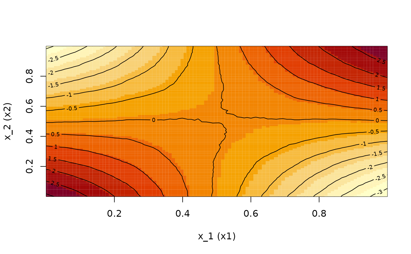
## Manually plot the ALE second-order effects of {x1, x2} and {x1, x4}
image(
  ALE.12$x.values[[1]], ALE.12$x.values[[2]], ALE.12$f.values, xlab = "x1",
  ylab = "x2", main = "(e)"
)
contour(
  ALE.12$x.values[[1]], ALE.12$x.values[[2]], ALE.12$f.values, add=TRUE,
  drawlabels=TRUE
)
image(
  ALE.14$x.values[[1]], ALE.14$x.values[[2]], ALE.14$f.values, xlab = "x1",
  ylab = "x4", main = "(f)"
)
contour(
  ALE.14$x.values[[1]], ALE.14$x.values[[2]], ALE.14$f.values, add=TRUE,
  drawlabels=TRUE
)

`ale` package equivalent

Now we demonstrate the same functionality with the ale package. We will work with the same model on the same data, so we will not create them again.

To create the model, we invoke the ALE() constructor which returns an ALE S7 object:

library(ale)
#> 
#> Attaching package: 'ale'
#> The following object is masked from 'package:base':
#> 
#>     get

nn_ale <- ALE(
  nnet.DAT, 
  data = DAT,
  pred_type = "raw",
  p_values = NULL
)

Here are some notable differences compared to ALEPlot:

Unlike {ALEPlot} that functions on only one variable at a time, ale generates ALE data for multiple variables in a dataset at once. By default, it generates ALE elements for all the individual predictor variables in the dataset that it is given (“first order” or 1D ALE); the user can specify a single variable or any subset of variables. We will cover more details in another vignette, but for our purposes here, we note the get() method can subsequently retrieve ALE data or plots for specific variables.
The ALE() constructor creates a default generic predict function that matches most standard R models. When the prediction type is not the default “response”, as in our case, the user can set the desired type with the pred_type argument. However, for more complex or non-standard prediction functions, ale supports custom functions with the pred_fun argument. See help(ALE) for details.

The plots can easily be printed out all at once by calling the plot() method. This generates an S7 ALEPlots object that contains all possible plots from the ALE data, along with convenient plot(), print(), and other methods. Simply calling plot() on the ALE object plots all the ALE plots together:

# Print plots
plot(nn_ale)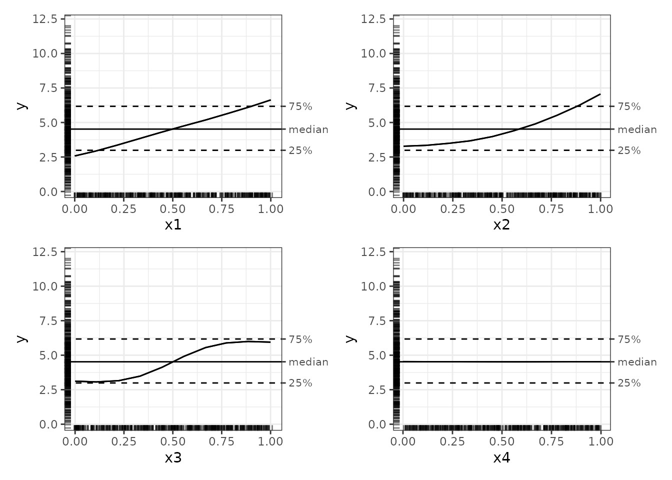

The plots in the ale package have numerous features that enhance interpretability:

The outcome y is displayed on its full original scale for context.
By default, plots are centred on the median, which is more intuitive than zero-centring because it is easier to see the effects of a variable relative to typical values. They can be centred on zero or on the mean with the ale_centre argument.
The 25% and 75% percentile markers show the middle 50% of the y values. Any ALE y value beyond these bands indicates that the x variable is so strong that it alone at the values indicated can shift the y value by that much.
Rug plots indicate the distribution of the data so that outliers are not over-interpreted.

It might not be clear that the previous plots display exactly the same data as those shown above from ALEPlot. To make the comparison clearer, we can plot the ALEs on a zero-centred scale:

# Zero-centred ALE plots
plot(nn_ale, ale_centre = 'zero')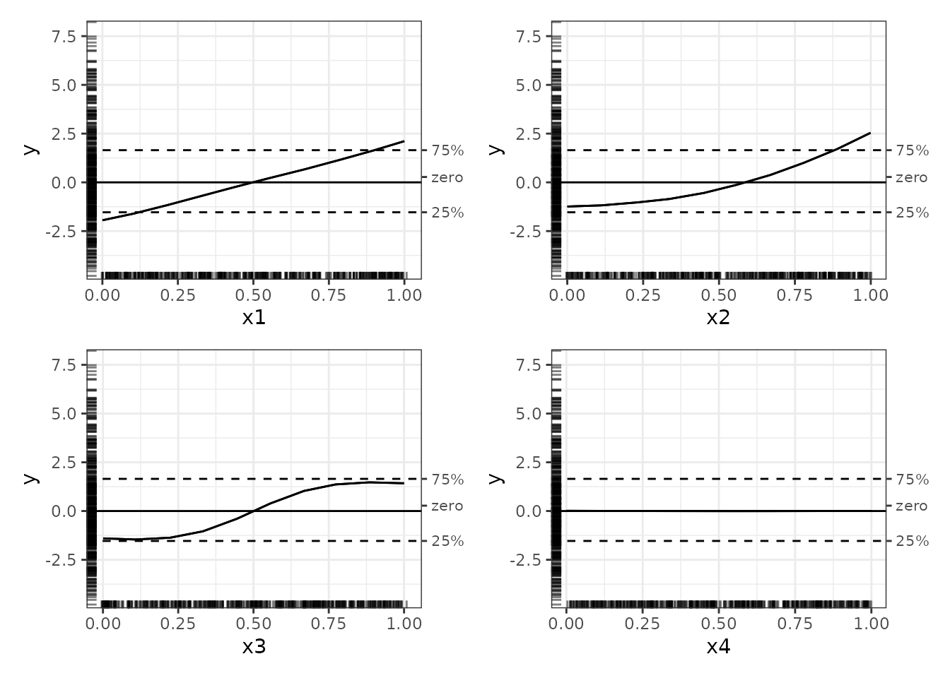

With these zero-centred plots, the full range of y values and the rug plots give some context that aids interpretation. (If the rugs look slightly different in each plot, it is because they are randomly jittered to avoid overplotting.)

The ale package also produces interaction plots; see the introductory vignette for details on how they are specified and created.

# Create and plot interactions
nn_ale_2D <- ALE(
  model = nnet.DAT, 
  x_cols = list(d2 = TRUE),
  data = DAT, 
  pred_type = "raw",
  p_values = NULL
)

# Print plots: plot() creates ALL possible plots from an ALE object
nnet_plots <- plot(nn_ale_2D)

print(nnet_plots, ncol = 2)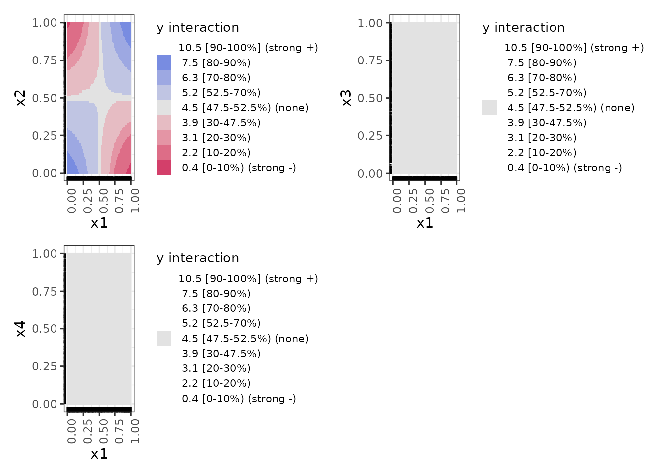

Here is a close-up of the x1 by x2 interaction plot:

# get() retrieves a specific desired plot
get(nnet_plots, 'x1:x2')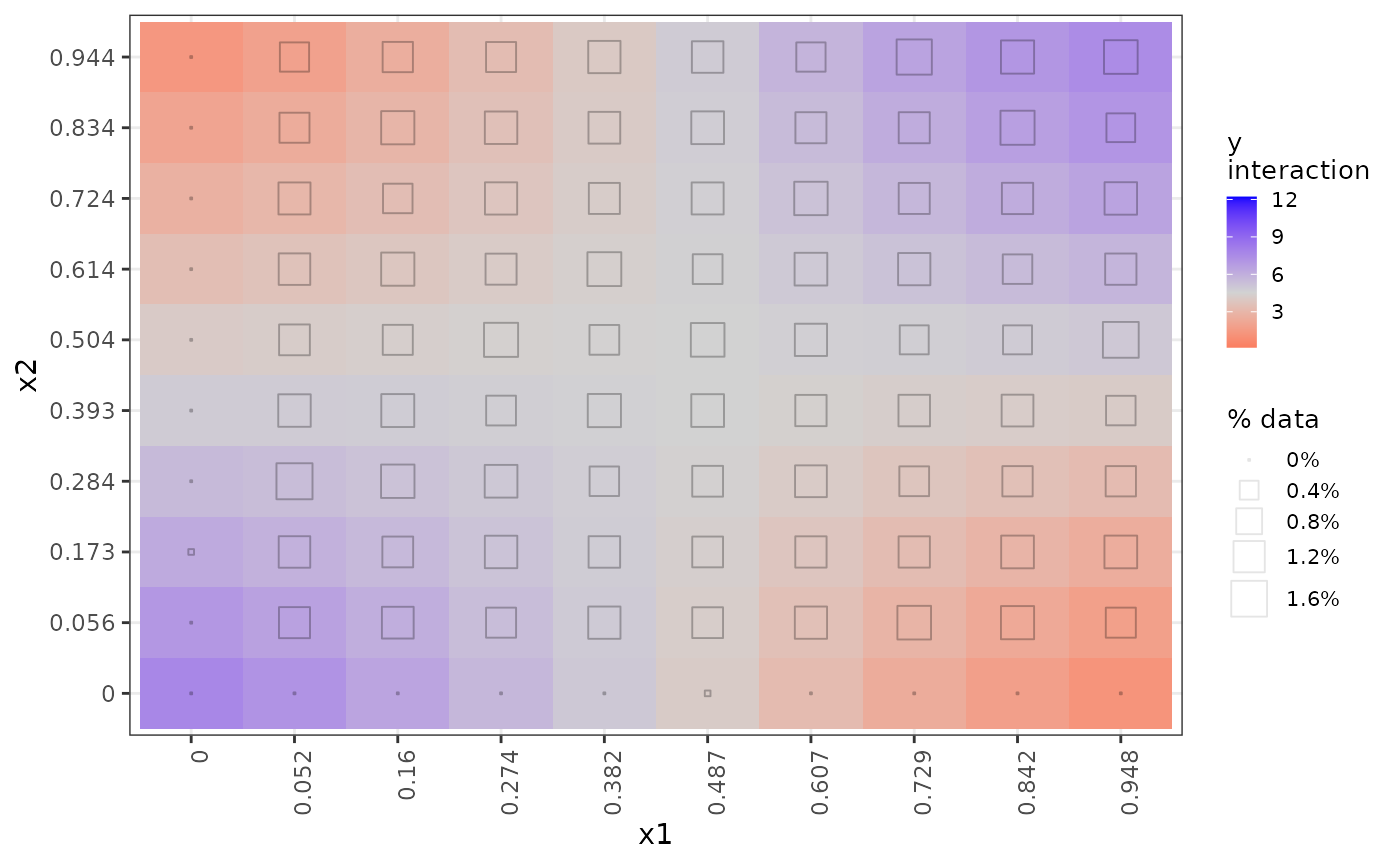

These interaction plots are heat maps that indicate the interaction regions that are above or below the average value of y with colour-blind–friendly colours on a diverging gradient. Blue indicates a positive interaction effect relative to the median; grey indicates no meaningful interaction; red indicates a negative effect. We find these easier to interpret than the contour maps from ALEPlot, especially since the colours in each plot are on the same scale and so the plots are directly comparable with each other. (The colour scheme is somewhat different when ALE statistics with p-values are calculated and plotted, which we do not present in this vignette.)

Rather than rug plots, the frequency of data in each interaction cell is indicated by a hollow square whose size varies with the percentage of data represented in the respective cell, as the legend “% data% indicates. In this synthetic dataset, most of the cells are equally represented with around 1.2% of the data; only the border cases have little or no data. This indication of data frequency is much more useful on real datasets as we have below where there are stark disparities in data representation in interaction cells.

The interpretation of these interaction plots is that in any given region, the interaction between x1 and x2 increases (blue) or decreases (red) y by the amount indicated over and above the separate individual direct effects of x1 and x2 shown in the 1D ALE plots above. It is not an indication of the total effect of both variables together but rather of the additional effect of their interaction beyond their individual effects. Thus, only the x1-x2 interaction shows any effect. For the interactions with x3, even though x3 indeed has a strong effect on y as we see in the 1D ALE plot above, it has no additional effect in interaction with the other variables, and so its interaction plots are entirely grey.

Real data with binary outcomes (ALEPlot Example 3)

The next code example from the {ALEPlot} package analyzes a real dataset with a binary outcome variable. Whereas the {ALEPlot} has the user load a CSV file that might not be readily available, we make that dataset available as the census dataset. We load it here with the adjustments necessary to run the {ALEPlot} example.

## R code for Example 3
## Load relevant packages
library(ALEPlot)
library(gbm, quietly = TRUE)
#> Loaded gbm 2.2.2
#> This version of gbm is no longer under development. Consider transitioning to gbm3, https://github.com/gbm-developers/gbm3

## Read data and fit a boosted tree supervised learning model
data(census, package = 'ale')  # load ale package version of the data
data <-  
  census |> 
  as.data.frame() |>   # ALEPlot is not compatible with the tibble format
  select(age:native_country, higher_income) |>  # Rearrange columns to match ALEPlot order
  stats::na.omit(data)

Although gradient boosted trees generally perform quite well, they are rather slow. So, we train this tree with only 600 trees rather than the 6000 from the original demo. Note that the model calls is based on data[,-c(3,4)], which drops the third and fourth variables (fnlwgt and education, respectively).

# Note: GBM training is rather slow
set.seed(0)
gbm.data <- gbm(
  higher_income ~ .,
  data = data[,-c(3,4)] |>
    # gbm::gbm() requires binary response outcomes to be numeric 0 or 1
    mutate(higher_income = as.integer(higher_income)),
  distribution = "bernoulli", 
  # the original demo trained 6000 trees; it is reduced here to 600 to be faster
  n.trees=600,  
  shrinkage=0.02,
  interaction.depth=3
)

gbm.data
#> gbm(formula = higher_income ~ ., distribution = "bernoulli", 
#>     data = mutate(data[, -c(3, 4)], higher_income = as.integer(higher_income)), 
#>     n.trees = 600, interaction.depth = 3, shrinkage = 0.02)
#> A gradient boosted model with bernoulli loss function.
#> 600 iterations were performed.
#> There were 12 predictors of which 12 had non-zero influence.

ALEPlot code

As before, we create a custom prediction function and then call the {ALEPlot} function to generate the plots. The prediction type here is “link”, which represents the log odds in the gbm package.

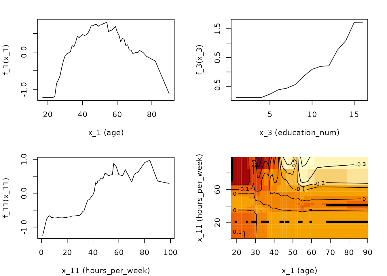
Creation of the ALE plots here is rather slow because the gbm predict function is slow. In this example, only age, education_num (number of years of education), and hours_per_week are plotted, along with the interaction between age and hours_per_week.

# Define the predictive function; note the additional arguments for the
# predict function in gbm.
yhat <- function(X.model, newdata) as.numeric(predict(
  X.model, newdata, n.trees = 600, type="link"
))

# Calculate and plot the ALE main and interaction effects for x_1, x_3,
# x_11, and {x_1, x_11}
par(mfrow = c(2,2), mar = c(4,4,2,2)+ 0.1)
ALE.1 <- ALEPlot(
  data[,-c(3,4,15)], gbm.data, pred.fun=yhat, J=1, K=100, NA.plot = TRUE
)
ALE.3 <- ALEPlot(
  data[,-c(3,4,15)], gbm.data, pred.fun=yhat, J=3, K=100, NA.plot = TRUE
)
ALE.11 <- ALEPlot(
  data[,-c(3,4,15)], gbm.data, pred.fun=yhat, J=11, K=100, NA.plot = TRUE
)
ALE.1and11 <- ALEPlot(
  data[,-c(3,4,15)], gbm.data, pred.fun=yhat, J=c(1,11), K=50, NA.plot = FALSE
)

`ale` package equivalent

Here is the analogous code using the ale package. In this case, we also need to define a custom predict function because of the particular n.trees argument. To speed things up in this vignette, we train only 600 trees rather than the 6000 from the original {ALEPlot} demonstration.

Log odds

We generate ALE for all 1D variables and for all 2D interactions involving age. However, we focus on age, education_num, and hours_per_week for comparison with {ALEPlot}. If the shapes of these plots look different, it is because ale tries as much as possible to display plots on the same y-axis coordinate scale for easy comparison across plots.

# Custom predict function that returns log odds
yhat_link <- function(object, newdata, type) {
    predict(object, newdata, type='link', n.trees = 600) |>  # return log odds
    as.numeric()
}

# Dump plots automatically generated by gbm into a temp PDF file so they don't print
pdf(file = NULL)
# Generate ALE data for all variables and age interactions.
# Note: this is rather slow because there are so many variables.
# However, the built-in parallelization speeds things up quite a bit.
gbm_ale_link <- ALE(
  gbm.data,
  x_cols = list(
    d1 = TRUE,      # all 1D ALE effects
    d2_all = 'age'  # only 2D interactions involving age
  ),  
  data = data,
  pred_fun = yhat_link,
  # Use fewer ALE bins so that interaction plots are easier to interpret
  max_num_bins = 10,  
  p_values = NULL
)

# Return to regular printing of plots
dev.off() |> invisible()

# Create an ALEPlots object with plots for all ALE data from the ALE object
gbm_link_plots <- plot(gbm_ale_link)

# Print only 1D ALE plots
gbm_link_plots |> 
  # Use subset() instead of get() to keep the special ALEPlots object 
  # plot and print functionality
  subset(list(d1 = TRUE)) |>  # 1D plots only
  print(ncol = 2)  # print in 2 columns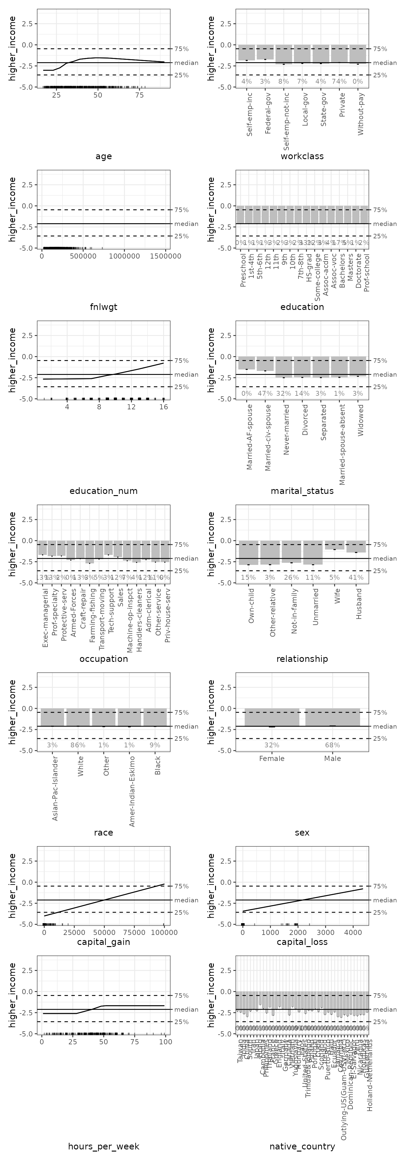

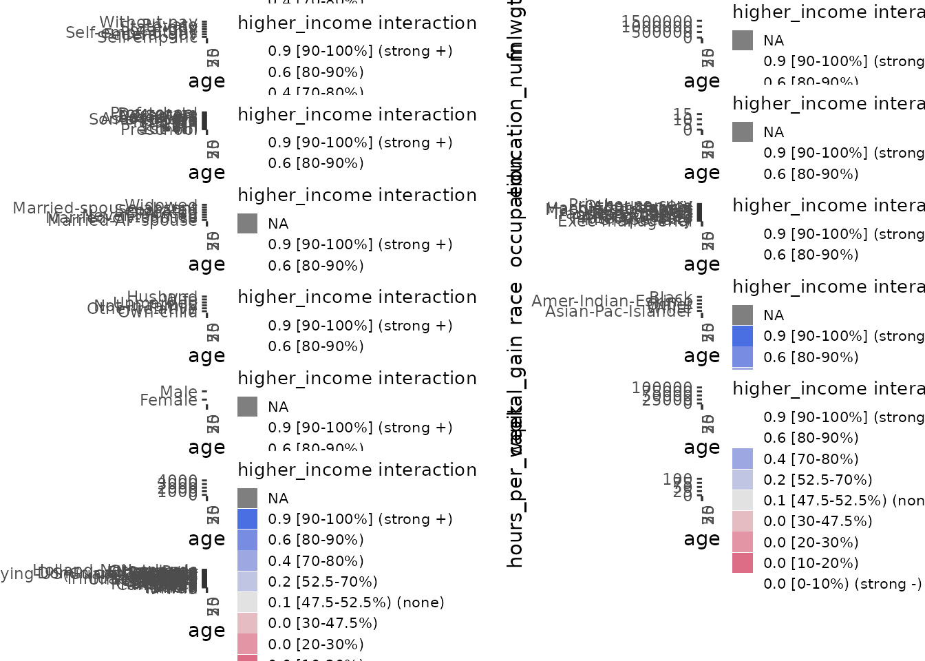
Now we plot all the 2D interactions involving age:

# Print only 2D ALE plots involving age
gbm_link_plots |> 
  # Use subset() instead of get() to keep the special ALEPlots object 
  # plot and print functionality
  subset(list(d2_all = 'age')) |>
  print(ncol = 1)  # print in 1 column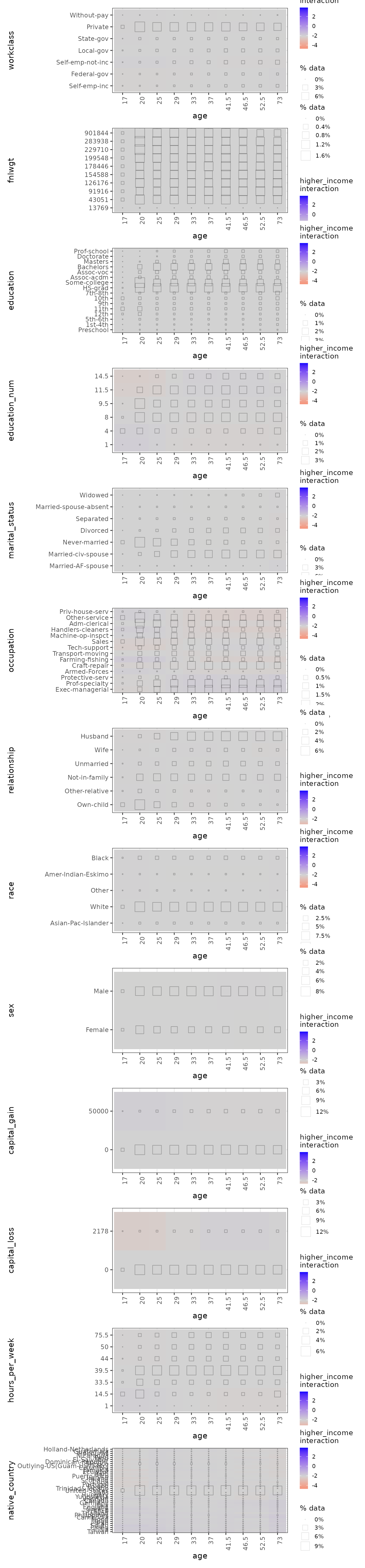

For direct comparison with {ALEPlot}, we can select the 1D plots for age, education_num, and hours_per_week, with the age-hours_per_week interaction. If the shapes of these plots look different, it is because ale tries as much as possible to display plots on the same y-axis coordinate scale for easy comparison across plots:

# Print only 2D ALE plots involving age
gbm_link_plots |> 
  # Use subset() instead of get() to keep the special ALEPlots object 
  # plot and print functionality
  get(~ age + education_num + hours_per_week + age:hours_per_week) |>
  purrr::list_flatten() |> 
  patchwork::wrap_plots()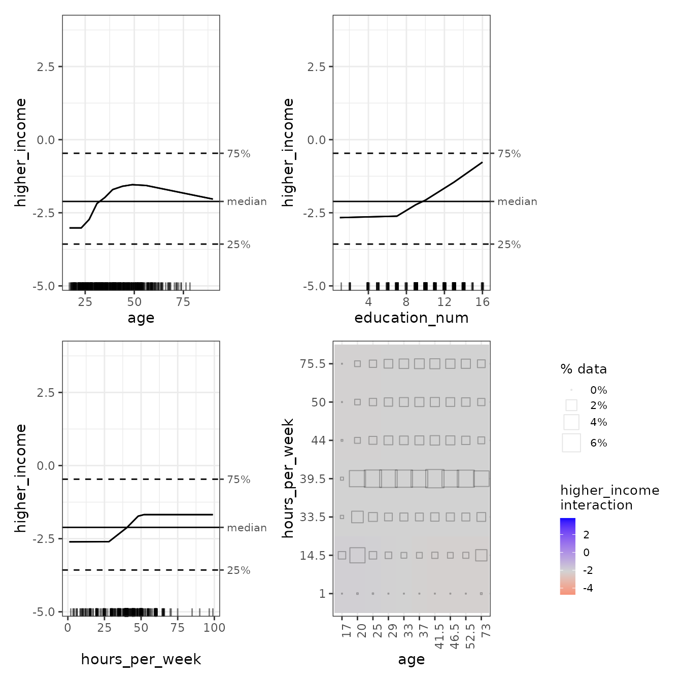

In the age:hours_per_week interaction plot, we can see that the interactions, if existent, are very week. The consistent-colour coding of the ale package makes this much clearer than the {ALEPlot} package.

Predicted probabilities

Log odds are not necessarily the most interpretable way to express probabilities (though we will show shortly that they are sometimes uniquely valuable). So, we repeat the ALE creation using the “response” prediction type for probabilities and the default median centring of the plots.

As we can see, the shapes of the plots are similar, but the y-axes are more easily interpretable as the probability (from 0 to 1) that a census respondent is in the higher income category. The median of around 10% or so indicates the median prediction of the GBM model: half of the respondents were predicted to have higher than a 10% likelihood of being higher income and half were predicted to have lower likelihood. The y-axis rug plots indicate that the GBM model predictions were generally rather extreme, either relatively close to 0 or 1, with few predictions in the middle.

# Custom predict function that returns probabilities
yhat_probs <- function(object, newdata, type) {
    predict(
      object, newdata, type = "response",  # return predicted probabilities
      n.trees = 600
    ) |>  # return log odds
    as.numeric()
}

# Dump plots automatically generated by gbm into a temp PDF file so they don't print
pdf(file = NULL)
# Generate ALE data for all variables and age interactions.
# Note: this is rather slow because there are so many variables.
# However, the built-in parallelization speeds things up quite a bit.
gbm_ale_probs <- ALE(
  gbm.data,
  x_cols = list(
    d1 = TRUE,      # all 1D ALE effects
    d2_all = 'age'  # only 2D interactions involving age
  ),  
  data = data,
  pred_fun = yhat_probs,
  # Use fewer ALE bins so that interaction plots are easier to interpret
  max_num_bins = 10,  
  p_values = NULL
)
# Return to regular printing of plots
dev.off() |> invisible()


# Create ALEPlots object with plots for all ALE data from the ALE object
gbm_probs_plots <- plot(gbm_ale_probs)

# Print only 1D ALE plots
gbm_probs_plots |> 
  # Use subset() instead of get() to keep the special ALEPlots object 
  # plot and print functionality
  subset(list(d1 = TRUE)) |>  # 1D plots only
  print(ncol = 2)  # print in 2 columns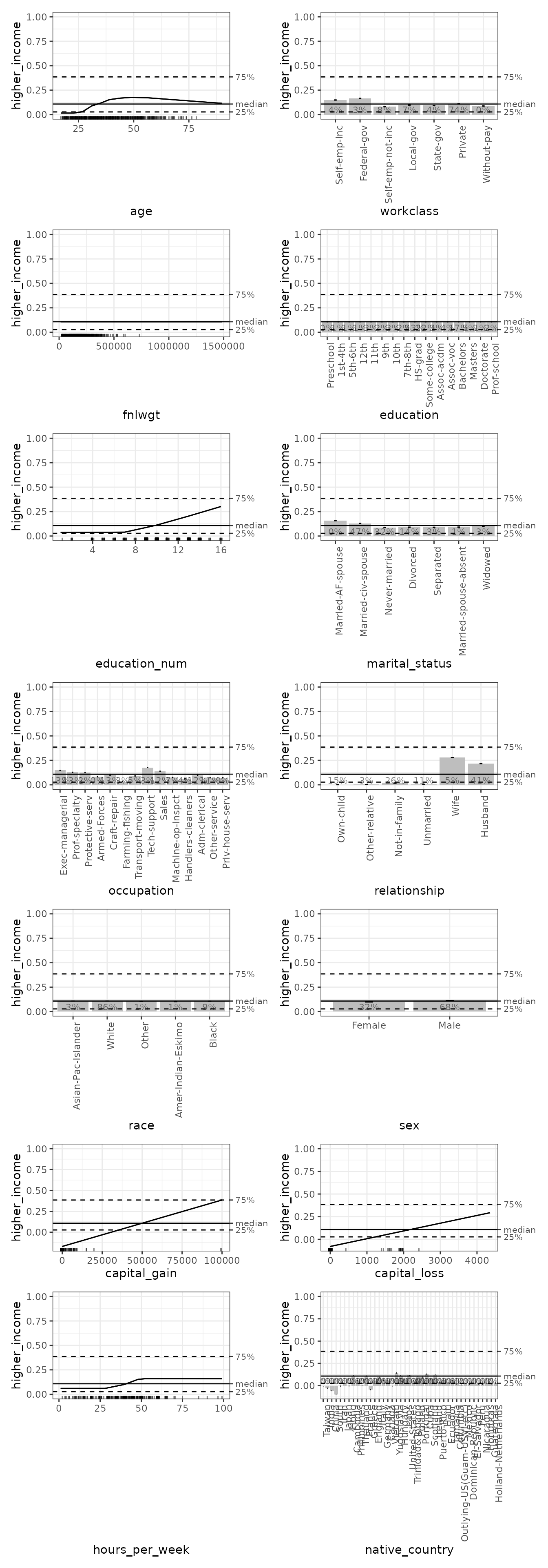

Finally, we again generate 2D interactions, this time based on probabilities instead of on log odds. However, probabilities might not be the best choice for indicating interactions because, as we see from the rugs in the 1D ALE plots, the GBM model heavily concentrates its probabilities in the extremes near 0 and 1. Thus, the plots’ suggestions of strong interactions are likely exaggerated. In this case, the log odds ALEs shown above are probably more relevant.

# Print only 2D ALE plots involving age
gbm_probs_plots |> 
  # Use subset() instead of get() to keep the special ALEPlots object 
  # plot and print functionality
  subset(list(d2_all = 'age')) |>
  print(ncol = 1)  # print in 1 column

Chitu Okoli

April 9, 2025

Simulated data with numeric outcomes (ALEPlot Example 2)

ALEPlot code

`ale` package equivalent

Real data with binary outcomes (ALEPlot Example 3)

ALEPlot code

`ale` package equivalent

Log odds

Predicted probabilities

Comparison between ALEPlot and ale packages

Chitu Okoli

April 9, 2025

Simulated data with numeric outcomes (ALEPlot Example 2)

ALEPlot code

ale package equivalent

Real data with binary outcomes (ALEPlot Example 3)

ALEPlot code

ale package equivalent

Log odds

Predicted probabilities

`ale` package equivalent

`ale` package equivalent