Random variable distributions of ALE statistics for generating p-values
Source:R/ALEpDist.R
ALEpDist.RdALE statistics are accompanied with two indicators of the confidence of their values. First, bootstrapping creates confidence intervals for ALE effects and ALE statistics to give a range of the possible ALE values. Second, we calculate p-values, an indicator of the probability that a given ALE statistic is random. An ALEpDist S7 object contains the necessary distribution data for generating such p-values.
Usage
ALEpDist(
  model,
  data = NULL,
  ...,
  y_col = NULL,
  rand_it = NULL,
  surrogate = FALSE,
  parallel = 0,
  model_packages = NULL,
  random_model_call_string = NULL,
  random_model_call_string_vars = character(),
  positive = TRUE,
  pred_fun = NULL,
  pred_type = "response",
  aled_fun = "mad",
  output_residuals = FALSE,
  seed = 0,
  silent = FALSE,
  .skip_validation = FALSE
)
Arguments
- model
See documentation for
ALE()- data
See documentation for
ALE()- ...
not used. Inserted to require explicit naming of subsequent arguments.
- y_col
See documentation for
ALE()- rand_it
non-negative integer(1). Number of times that the model should be retrained with a new random variable. The default of
NULLwill generate 1000 iterations, which should give reasonably stable p-values; these are considered "exact" p-values. It can be reduced for approximate ("approx") p-values as low as 100 for faster test runs but then the p-values are not as stable.rand_itbelow 100 is not allowed as such p-values are inaccurate.- surrogate
logical(1). Create p-value distributions based on a surrogate linear model (
TRUE) instead of on the originalmodel(defaultFALSE). Note that while faster surrogate p-values are convenient for interactive analysis, they are not acceptable for definitive conclusions or publication. See details.- parallel
See documentation for
ALE(). Note that for exact p-values, by default 1000 random variables are trained. So, even with parallel processing, the procedure is very slow.- model_packages
See documentation for
ALE()- random_model_call_string
character(1). If
NULL, theALEpDist()constructor tries to automatically detect and construct the call for p-values. If it cannot, the constructor will fail. In that case, a character string of the full call for the model must be provided that includes the random variable. See details.- random_model_call_string_vars
See documentation for
model_call_string_varsinModelBoot(); their operation is very similar.- positive
See documentation for
ModelBoot()- pred_fun, pred_type
See documentation for
ALE()- aled_fun
See documentation for
ALE()- output_residuals
logical(1). If
TRUE, returns the residuals in addition to the raw data of the generated random statistics (which are always returned). The defaultFALSEdoes not return the residuals.- seed
See documentation for
ALE()- silent
See documentation for
ALE()- .skip_validation
Internal use only. logical(1). Skip non-mutating data validation checks. Changing the default
FALSErisks crashing with incomprehensible error messages.
Value
An object of class ALEpDist with properties rand_stats, residual_distribution, residuals, and params.
Properties
- rand_stats
A named list of tibbles. There is normally one element whose name is the same as
y_colexcept ify_colis a categorical variable; in that case, the elements are named for each category ofy_col. Each element is a tibble whose rows are each of therand_it_okiterations of the random variable analysis and whose columns are the ALE statistics obtained for each random variable.- residual_distribution
A
univariateMLobject with the closest estimated distribution for theresidualsas determined byunivariateML::model_select(). This is the distribution used to generate all the random variables.- residuals
If
output_residuals == TRUE, returns a matrix of the actualy_colvalues fromdataminus the predicted values from themodel(without random variables) on thedata. The rows correspond to each row ofdata. The columns correspond to the named elements (y_color categories) described above forrand_stats.NULLifoutput_residuals == FALSE(default).- params
Parameters used to generate p-value distributions. Most of these repeat selected arguments passed to
ALEpDist(). These are either values provided by the user or used by default if the user did not change them but the following additional or modified objects are notable:* `model`: selected elements that describe the `model` used to generate the random distributions. * `rand_it`: the number of random iterations requested by the user either explicitly (by specifying a whole number) or implicitly with the default `NULL`: exact p distributions imply 1000 iterations and surrogate distributions imply 100 unless an explicit number of iterations is requested. * `rand_it_ok`: A whole number with the number of `rand_it` iterations that successfully generated a random variable, that is, those that did not fail for whatever reason. The `rand_it` - `rand_it_ok` failed attempts are discarded. * `exactness`: A string. For regular p-values generated from the original model, `'exact'` if `rand_it_ok >= 1000` and `'approx'` otherwise. `'surrogate'` for p-values generated from a surrogate model. `'invalid'` if `rand_it_ok < 100`. * `probs_inverted`: `TRUE` if the original probability values of the `ALEpDist` object have been inverted. This is accomplished using [invert_probs()] on an `ALE` object. `FALSE`, `NULL`, or absent otherwise.
Exact p-values for ALE statistics
Because ALE is non-parametric (that is, it does not assume any particular distribution of data), the {ale} package takes a literal frequentist approach to the calculation of empirical (Monte Carlo) p-values. That is, it literally retrains the model 1000 times, each time modifying it by adding a distinct random variable to the model. (The number of iterations is customizable with the rand_it argument.) The ALEs and ALE statistics are calculated for each random variable. The percentiles of the distribution of these random-variable ALEs are then used to determine p-values for non-random variables. Thus, p-values are interpreted as the frequency of random variable ALE statistics that exceed the value of ALE statistic of the actual variable in question. The specific steps are as follows:
The residuals of the original model trained on the training data are calculated (residuals are the actual y target value minus the predicted values).
The closest distribution of the residuals is detected with
univariateML::model_select().1000 new models are trained by generating a random variable each time with
univariateML::rml()and then training a new model with that random variable added.The ALEs and ALE statistics are calculated for each random variable.
For each ALE statistic, the empirical cumulative distribution function (
stats::ecdf()) is used to create a function to determine p-values according to the distribution of the random variables' ALE statistics.
Because the ale package is model-agnostic (that is, it works with any kind of R model), the ALEpDist() constructor cannot always automatically manipulate the model object to create the p-values. It can only do so for models that follow modelling conventions similar to those of base R algorithms (like stats::lm() and stats::glm()) and many widely used statistics packages (like mgcv and survival), but probably not for most machine learning algorithms (like tidymodels and caret). For algorithms that do not follow base R conventions, the user needs to do a little work to help the ALEpDist() constructor correctly manipulate its model object:
The full model call must be passed as a character string in the argument
random_model_call_string, with two slight modifications as follows.In the formula that specifies the model, you must add a variable named 'random_variable'. This corresponds to the random variables that the constructor will use to estimate p-values.
The dataset on which the model is trained must be named 'rand_data'. This corresponds to the modified datasets that will be used to train the random variables.
See the example below for how this is implemented.
If the model generation is unstable (because of a small dataset size or a finicky model algorithm), then one or more iterations might fail, possibly dropping the number of successful iterations to below 1000. Then the p-values are only considered approximate; they are no longer exact. If that is the case, then request rand_it at a sufficiently high number such that even if some iterations fail, at least 1000 will succeed. For example, for an ALEpDist object named p_dist, if p_dist@params$rand_it_ok is 950, you could rerun ALEpDist() with rand_it = 1100 or higher to allow for up to 100 possible failures.
Faster approximate and surrogate p-values
The procedure we have just described requires at least 1000 random iterations for p-values to be considered "exact". Unfortunately, this procedure is rather slow–it takes at least 1000 times as long as the time it takes to train the model once.
With fewer iterations (at least 100), p-values can only be considered approximate ("approx"). Fewer than 100 such p-values are invalid. There might be fewer iterations either because the user requests them with the rand_it argument or because some iterations fail for whatever reason. As long as at least 1000 iterations succeed, p-values will be considered exact.
Because the procedure can be very slow, a faster version of the algorithm generates "surrogate" p-values by substituting the original model with a linear model that predicts the same y_col outcome from all the other columns in data. By default, these surrogate p-values use only 100 iterations and if the dataset is large, the surrogate model samples 1000 rows. Thus, the surrogate p-values can be generated much faster than for slower model algorithms on larger datasets. Although they are suitable for model development and analysis because they are faster to generate, they are less reliable than approximate p-values based on the original model. In any case, definitive conclusions (e.g., for publication) always require exact p-values with at least 1000 iterations on the original model. Note that surrogate p-values are always marked as "surrogate"; even if they are generated based on over 1000 iterations, they can never be considered exact because they are not based on the original model.
References
Okoli, Chitu. 2023. "Statistical Inference Using Machine Learning and Classical Techniques Based on Accumulated Local Effects (ALE)." arXiv. doi:10.48550/arXiv.2310.09877.
Examples
# \donttest{
library(dplyr)
# Load diamonds dataset with some cleanup
diamonds <- ggplot2::diamonds |>
filter(!(x == 0 | y == 0 | z == 0)) |>
# https://lorentzen.ch/index.php/2021/04/16/a-curious-fact-on-the-diamonds-dataset/
distinct(
price, carat, cut, color, clarity,
.keep_all = TRUE
) |>
rename(
x_length = x,
y_width = y,
z_depth = z,
depth_pct = depth
)
# Create a GAM model with flexible curves to predict diamond price
# Smooth all numeric variables and include all other variables
# Build the model on training data, not on the full dataset.
gam_diamonds <- mgcv::gam(
price ~ s(carat) + s(depth_pct) + s(table) + s(x_length) + s(y_width) + s(z_depth) +
cut + color + clarity,
data = diamonds
)
summary(gam_diamonds)
#>
#> Family: gaussian
#> Link function: identity
#>
#> Formula:
#> price ~ s(carat) + s(depth_pct) + s(table) + s(x_length) + s(y_width) +
#> s(z_depth) + cut + color + clarity
#>
#> Parametric coefficients:
#> Estimate Std. Error t value Pr(>|t|)
#> (Intercept) 4436.199 13.315 333.165 < 2e-16 ***
#> cut.L 263.124 39.117 6.727 1.76e-11 ***
#> cut.Q 1.792 27.558 0.065 0.948151
#> cut.C 74.074 20.169 3.673 0.000240 ***
#> cut^4 27.694 14.373 1.927 0.054004 .
#> color.L -2152.488 18.996 -113.313 < 2e-16 ***
#> color.Q -704.604 17.385 -40.528 < 2e-16 ***
#> color.C -66.839 16.366 -4.084 4.43e-05 ***
#> color^4 80.376 15.289 5.257 1.47e-07 ***
#> color^5 -110.164 14.484 -7.606 2.89e-14 ***
#> color^6 -49.565 13.464 -3.681 0.000232 ***
#> clarity.L 4111.691 33.499 122.742 < 2e-16 ***
#> clarity.Q -1539.959 31.211 -49.341 < 2e-16 ***
#> clarity.C 762.680 27.013 28.234 < 2e-16 ***
#> clarity^4 -232.214 21.977 -10.566 < 2e-16 ***
#> clarity^5 193.854 18.324 10.579 < 2e-16 ***
#> clarity^6 46.812 16.172 2.895 0.003799 **
#> clarity^7 132.621 14.274 9.291 < 2e-16 ***
#> ---
#> Signif. codes: 0 ‘***’ 0.001 ‘**’ 0.01 ‘*’ 0.05 ‘.’ 0.1 ‘ ’ 1
#>
#> Approximate significance of smooth terms:
#> edf Ref.df F p-value
#> s(carat) 8.695 8.949 37.027 < 2e-16 ***
#> s(depth_pct) 7.606 8.429 6.758 < 2e-16 ***
#> s(table) 5.759 6.856 3.682 0.000736 ***
#> s(x_length) 8.078 8.527 60.936 < 2e-16 ***
#> s(y_width) 7.477 8.144 211.202 < 2e-16 ***
#> s(z_depth) 9.000 9.000 16.266 < 2e-16 ***
#> ---
#> Signif. codes: 0 ‘***’ 0.001 ‘**’ 0.01 ‘*’ 0.05 ‘.’ 0.1 ‘ ’ 1
#>
#> R-sq.(adj) = 0.929 Deviance explained = 92.9%
#> GCV = 1.2602e+06 Scale est. = 1.2581e+06 n = 39739
# For speed, these examples use retrieve_rds() to load pre-created objects
# from an online repository.
# To run the code yourself, execute the code blocks directly.
serialized_objects_site <- "https://github.com/tripartio/ale/raw/main/download"
# Generating p_value distribution objects is slow because it retrains the model 100 times,
# so this example loads a pre-created ALEpDist object.
p_dist_gam_diamonds <- retrieve_rds(
c(serialized_objects_site, 'p_dist_gam_diamonds_readme.0.5.2.rds'),
{
# To run the code yourself, execute this code block directly.
ALEpDist(
gam_diamonds, diamonds,
# Normally should be default 1000, but just 100 for quicker demo
rand_it = 100
)
}
)
# Examine the structure of the returned object
print(p_dist_gam_diamonds)
#> <ale::ALEpDist>
#> @ rand_stats :List of 1
#> .. $ price: tibble [100 × 6] (S3: tbl_df/tbl/data.frame)
#> .. ..$ aled : num [1:100] 4.07 6.15 7.69 8.13 2.26 ...
#> .. ..$ aler_min : num [1:100] -55.2 -227.8 -398.2 -637.2 -82.7 ...
#> .. ..$ aler_max : num [1:100] 307.8 187.6 237.5 226.4 59.3 ...
#> .. ..$ naled : num [1:100] 0.0531 0.0745 0.089 0.0904 0.0321 ...
#> .. ..$ naler_min: num [1:100] -0.576 -2.257 -3.865 -6.049 -0.808 ...
#> .. ..$ naler_max: num [1:100] 2.733 1.696 2.151 2.041 0.581 ...
#> @ residual_distribution: 'univariateML' Named num [1:4] 22.86 1372.41 2.67 1.34
#> .. - attr(*, "logLik")= num -329520
#> .. - attr(*, "call")= language f(x = x, na.rm = na.rm)
#> .. - attr(*, "n")= int 39739
#> .. - attr(*, "model")= chr "Skew Student-t"
#> .. - attr(*, "density")= chr "fGarch::dsstd"
#> .. - attr(*, "support")= num [1:2] -Inf Inf
#> .. - attr(*, "names")= chr [1:4] "mean" "sd" "nu" "xi"
#> .. - attr(*, "default")= num [1:4] 0 1 3 2
#> .. - attr(*, "continuous")= logi TRUE
#> @ residuals : NULL
#> @ params :List of 11
#> .. $ model :List of 4
#> .. ..$ class : chr [1:3] "gam" "glm" "lm"
#> .. ..$ call : chr "mgcv::gam(formula = price ~ s(carat) + s(depth_pct) + s(table) + \n s(x_length) + s(y_width) + s(z_depth) + "| __truncated__
#> .. ..$ print : chr "\nFamily: gaussian \nLink function: identity \n\nFormula:\nprice ~ s(carat) + s(depth_pct) + s(table) + s(x_len"| __truncated__
#> .. ..$ summary: chr "\nFamily: gaussian \nLink function: identity \n\nFormula:\nprice ~ s(carat) + s(depth_pct) + s(table) + s(x_len"| __truncated__
#> .. $ y_col : chr "price"
#> .. $ rand_it : num 100
#> .. $ parallel : Named int 22
#> .. ..- attr(*, "names")= chr "system"
#> .. $ model_packages : chr "mgcv"
#> .. $ random_model_call_string : NULL
#> .. $ random_model_call_string_vars: chr(0)
#> .. $ positive : logi TRUE
#> .. $ seed : num 0
#> .. $ rand_it_ok : int 100
#> .. $ exactness : chr "approx"
# Calculate ALEs with p-values
ale_gam_diamonds <- retrieve_rds(
# For speed, load a pre-created object by default.
c(serialized_objects_site, 'ale_gam_diamonds_stats_readme.0.5.2.rds'),
{
# To run the code yourself, execute this code block directly.
ALE(
gam_diamonds,
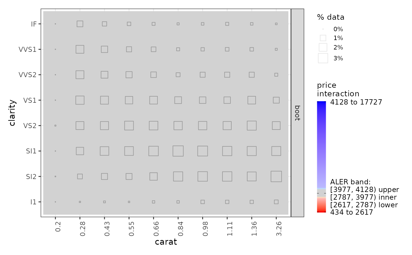
# generate ALE for all 1D variables and the carat:clarity 2D interaction,
x_cols = list(d1 = TRUE, d2 = 'carat:clarity'),
data = diamonds,
p_values = p_dist_gam_diamonds,
# Usually at least 100 bootstrap iterations, but just 10 here for a faster demo
boot_it = 10
)
}
)
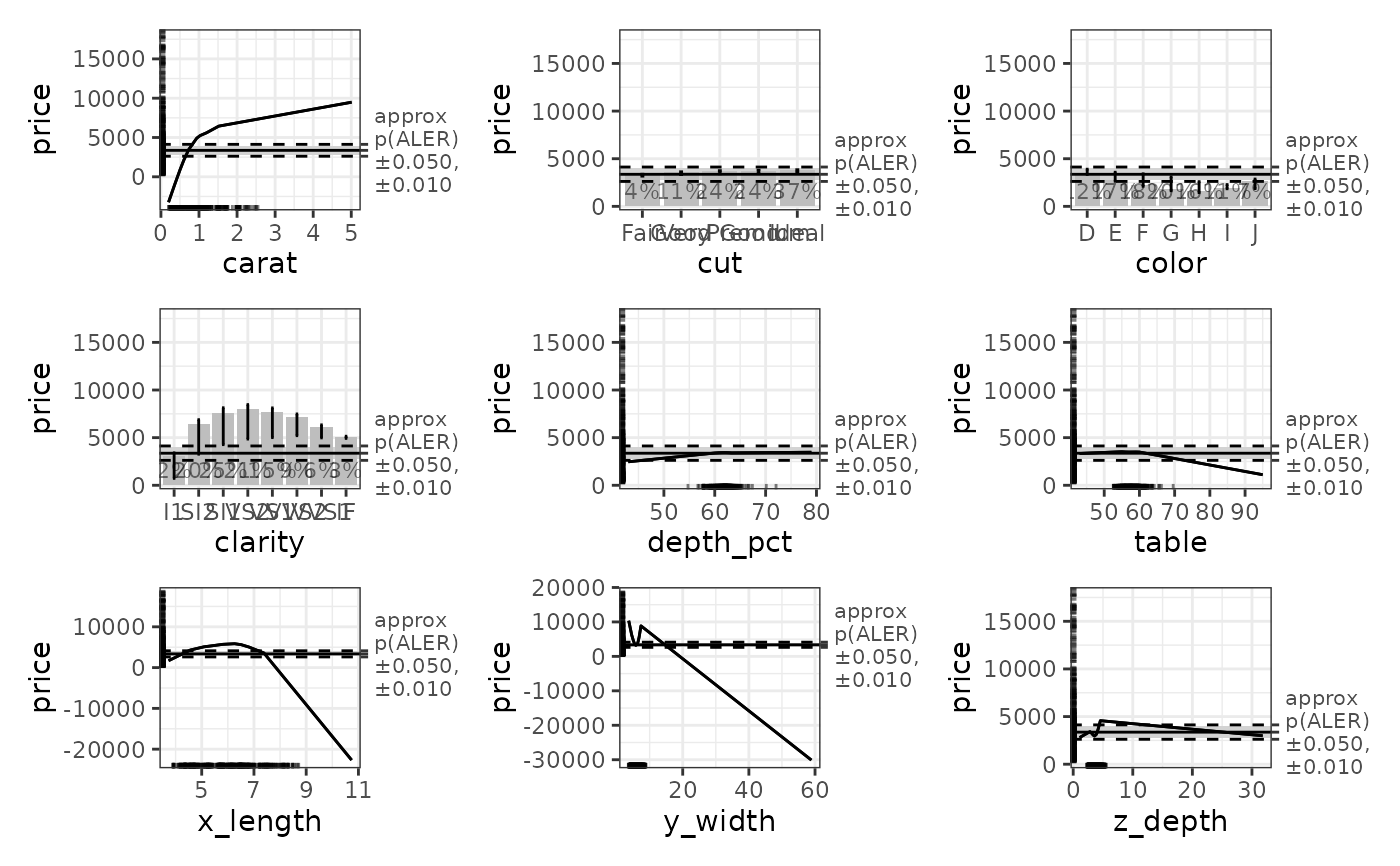
# Plot the ALE data. The horizontal bands in the plots use the p-values.
plot(ale_gam_diamonds)
 # For models that give errors with the default settings,
# you can use 'random_model_call_string' to specify a model for the estimation
# of p-values from random variables as in this example.
# See details above for an explanation.
pd_diamonds_special <- retrieve_rds(
# For speed, load a pre-created object by default.
c(serialized_objects_site, 'pd_diamonds_special.0.5.2.rds'),
{
# To run the code yourself, execute this code block directly.
ALEpDist(
gam_diamonds,
diamonds,
random_model_call_string = 'mgcv::gam(
price ~ s(carat) + s(depth_pct) + s(table) + s(x_length) + s(y_width) + s(z_depth) +
cut + color + clarity + random_variable,
data = rand_data
)',
# Normally should be default 1000, but just 100 for quicker demo
rand_it = 100
)
}
)
#> Warning: cannot open URL 'https://github.com/tripartio/ale/raw/main/download/pd_diamonds_special.0.5.2.rds': HTTP status was '404 Not Found'
# saveRDS(pd_diamonds_special, file.choose())
# Examine the structure of the returned object
print(pd_diamonds_special)
#> <ale::ALEpDist>
#> @ rand_stats :List of 1
#> .. $ price: tibble [100 × 6] (S3: tbl_df/tbl/data.frame)
#> .. ..$ aled : num [1:100] 4.07 6.15 7.69 8.13 2.26 ...
#> .. ..$ aler_min : num [1:100] -55.2 -227.8 -398.2 -637.2 -82.7 ...
#> .. ..$ aler_max : num [1:100] 307.8 187.6 237.5 226.4 59.3 ...
#> .. ..$ naled : num [1:100] 0.0531 0.0745 0.089 0.0904 0.0321 ...
#> .. ..$ naler_min: num [1:100] -0.576 -2.257 -3.865 -6.049 -0.808 ...
#> .. ..$ naler_max: num [1:100] 2.733 1.696 2.151 2.041 0.581 ...
#> @ residual_distribution: 'univariateML' Named num [1:4] 22.86 1372.41 2.67 1.34
#> .. - attr(*, "logLik")= num -329520
#> .. - attr(*, "call")= language f(x = x, na.rm = na.rm)
#> .. - attr(*, "n")= int 39739
#> .. - attr(*, "model")= chr "Skew Student-t"
#> .. - attr(*, "density")= chr "fGarch::dsstd"
#> .. - attr(*, "support")= num [1:2] -Inf Inf
#> .. - attr(*, "names")= chr [1:4] "mean" "sd" "nu" "xi"
#> .. - attr(*, "default")= num [1:4] 0 1 3 2
#> .. - attr(*, "continuous")= logi TRUE
#> @ residuals : NULL
#> @ params :List of 12
#> .. $ model :List of 2
#> .. ..$ class: chr [1:3] "gam" "glm" "lm"
#> .. ..$ hash : chr "e92e511307cb9457ffafbe991e2738f3"
#> .. $ y_col : chr "price"
#> .. $ rand_it : num 100
#> .. $ parallel : num 0
#> .. $ model_packages : NULL
#> .. $ random_model_call_string : chr "mgcv::gam(\n price ~ s(carat) + s(depth_pct) + s(table) + s(x_length) + s(y_width) + s(z_depth) +\n "| __truncated__
#> .. $ random_model_call_string_vars: chr(0)
#> .. $ positive : logi TRUE
#> .. $ aled_fun : chr "mad"
#> .. $ seed : num 0
#> .. $ rand_it_ok : int 100
#> .. $ exactness : chr "approx"
# }
# For models that give errors with the default settings,
# you can use 'random_model_call_string' to specify a model for the estimation
# of p-values from random variables as in this example.
# See details above for an explanation.
pd_diamonds_special <- retrieve_rds(
# For speed, load a pre-created object by default.
c(serialized_objects_site, 'pd_diamonds_special.0.5.2.rds'),
{
# To run the code yourself, execute this code block directly.
ALEpDist(
gam_diamonds,
diamonds,
random_model_call_string = 'mgcv::gam(
price ~ s(carat) + s(depth_pct) + s(table) + s(x_length) + s(y_width) + s(z_depth) +
cut + color + clarity + random_variable,
data = rand_data
)',
# Normally should be default 1000, but just 100 for quicker demo
rand_it = 100
)
}
)
#> Warning: cannot open URL 'https://github.com/tripartio/ale/raw/main/download/pd_diamonds_special.0.5.2.rds': HTTP status was '404 Not Found'
# saveRDS(pd_diamonds_special, file.choose())
# Examine the structure of the returned object
print(pd_diamonds_special)
#> <ale::ALEpDist>
#> @ rand_stats :List of 1
#> .. $ price: tibble [100 × 6] (S3: tbl_df/tbl/data.frame)
#> .. ..$ aled : num [1:100] 4.07 6.15 7.69 8.13 2.26 ...
#> .. ..$ aler_min : num [1:100] -55.2 -227.8 -398.2 -637.2 -82.7 ...
#> .. ..$ aler_max : num [1:100] 307.8 187.6 237.5 226.4 59.3 ...
#> .. ..$ naled : num [1:100] 0.0531 0.0745 0.089 0.0904 0.0321 ...
#> .. ..$ naler_min: num [1:100] -0.576 -2.257 -3.865 -6.049 -0.808 ...
#> .. ..$ naler_max: num [1:100] 2.733 1.696 2.151 2.041 0.581 ...
#> @ residual_distribution: 'univariateML' Named num [1:4] 22.86 1372.41 2.67 1.34
#> .. - attr(*, "logLik")= num -329520
#> .. - attr(*, "call")= language f(x = x, na.rm = na.rm)
#> .. - attr(*, "n")= int 39739
#> .. - attr(*, "model")= chr "Skew Student-t"
#> .. - attr(*, "density")= chr "fGarch::dsstd"
#> .. - attr(*, "support")= num [1:2] -Inf Inf
#> .. - attr(*, "names")= chr [1:4] "mean" "sd" "nu" "xi"
#> .. - attr(*, "default")= num [1:4] 0 1 3 2
#> .. - attr(*, "continuous")= logi TRUE
#> @ residuals : NULL
#> @ params :List of 12
#> .. $ model :List of 2
#> .. ..$ class: chr [1:3] "gam" "glm" "lm"
#> .. ..$ hash : chr "e92e511307cb9457ffafbe991e2738f3"
#> .. $ y_col : chr "price"
#> .. $ rand_it : num 100
#> .. $ parallel : num 0
#> .. $ model_packages : NULL
#> .. $ random_model_call_string : chr "mgcv::gam(\n price ~ s(carat) + s(depth_pct) + s(table) + s(x_length) + s(y_width) + s(z_depth) +\n "| __truncated__
#> .. $ random_model_call_string_vars: chr(0)
#> .. $ positive : logi TRUE
#> .. $ aled_fun : chr "mad"
#> .. $ seed : num 0
#> .. $ rand_it_ok : int 100
#> .. $ exactness : chr "approx"
# }