Introduction
The ale package creates plots with several elements to help us interpret accumulated local effects. Sometimes, we want to focus on a particular range of values or adapt the appearance of the plots. The customize() function lets us make these changes to one or more plots in an ALEPlots object.
This article demonstrates how to select plots to customize, zoom on their axes, and add ggplot2 layers. You should first read the introductory vignette for an explanation of ALE and the basic functionality of the package.
The workflow is to create an ALE object, call plot() to generate an ALEPlots object, customize the plots, and then print them. Customization changes the presentation of existing ALE results; it does not refit the model or recalculate ALE. We will keep the original plots so that we can compare each customization with the starting point.
Prepare the diamonds example
For our illustration, we train a random forest On the diamonds dataset. We begin by loading the necessary libraries.
The following object is masked from 'package:base':

    get
# Enable parallelization of the ALE package (set to the number of threads you want)
options(ale.parallel = 2)

library(dplyr)
Attaching package: 'dplyr'
The following objects are masked from 'package:stats':

    filter, lag
The following objects are masked from 'package:base':

    intersect, setdiff, setequal, union
library(ggplot2)

# For speed, these examples use retrieve_rds() to load pre-created objects
# from an online repository.
# To run the code yourself, execute the code blocks directly.
serialized_objects_site <- "https://github.com/tripartio/ale/raw/wip/download"
The diamonds dataset is included with ggplot2. We first remove invalid entries and duplicates, and give the physical dimensions more descriptive names.
diamonds <- ggplot2::diamonds |>
  filter(!(x == 0 | y == 0 | z == 0)) |>
  # https://lorentzen.ch/index.php/2021/04/16/a-curious-fact-on-the-diamonds-dataset/
  distinct(
    price, carat, cut, color, clarity,
    .keep_all = TRUE
  ) |>
  rename(
    x_length = x,
    y_width = y,
    z_depth = z,
    depth_pct = depth
  )
We train a random forest to predict diamond prices. The forest uses all the predictors; we will select just three of them for the ALE demonstration.
rf_diamonds <- ranger::ranger(
  price ~ ., diamonds,  # train for IML on full dataset
  mtry = 7,  # number of variables per tree
  min.node.size = 4,  # minimum leaf (terminal node) size
  sample.fraction = 0.465,  # fraction of rows to sample
  num.trees = 50,  # small forest for a faster demonstration
  seed = 0
)
Next, we create ALE data to explain this random forest. For this demonstration, we will focus on just three predictors: carat (weight), cut (an ordered factor describing cut quality), and x_length (length in millimetres). We request their three 1D main effects and all three pairwise 2D interactions:
# Create ALE data
# # To run the slow code yourself, uncomment and execute this code block directly.
# ale_rf_diamonds <- ALE(
#   rf_diamonds,
#   data = diamonds,
#   x_cols = ~ carat + cut + x_length +
#     carat:cut + carat:x_length + cut:x_length
# )


ale_rf_diamonds <- serialized_objects_site |>
  file.path('ale_rf_diamonds_custom_plots.0.6.0.rds') |>
  url() |>
  readRDS()
Now, we create an ALEPlots object to generate and manipulate ALE plots:
# Generate an ALEPlots object and keep it as our starting point.
diamonds_plots <- ale_rf_diamonds |>
  plot()
The print() method displays 1D and 2D plots separately. We can use subset() to display just one set at a time.
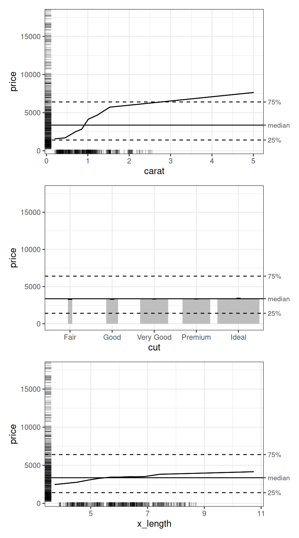
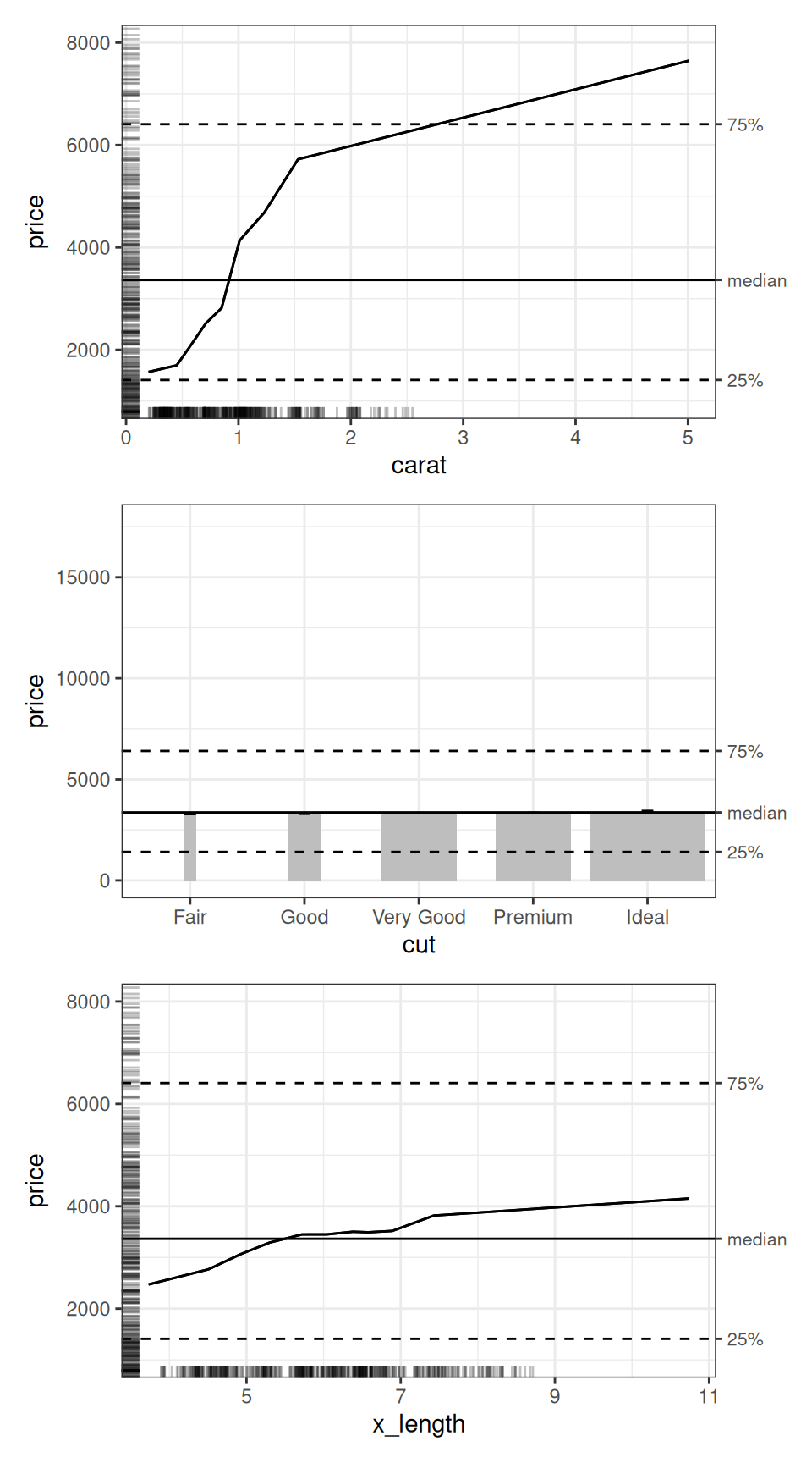
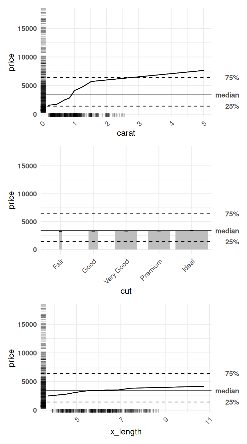
The numeric predictors have line charts, while cut has a column chart. The column widths reflect the relative numbers of observations in each level of cut. By default, the ALE curves are centred on the median diamond price. Thus, the y-axis is on the price scale in US dollars, rather than centred on zero. The horizontal lines mark the median and the 25th and 75th percentiles of observed prices.
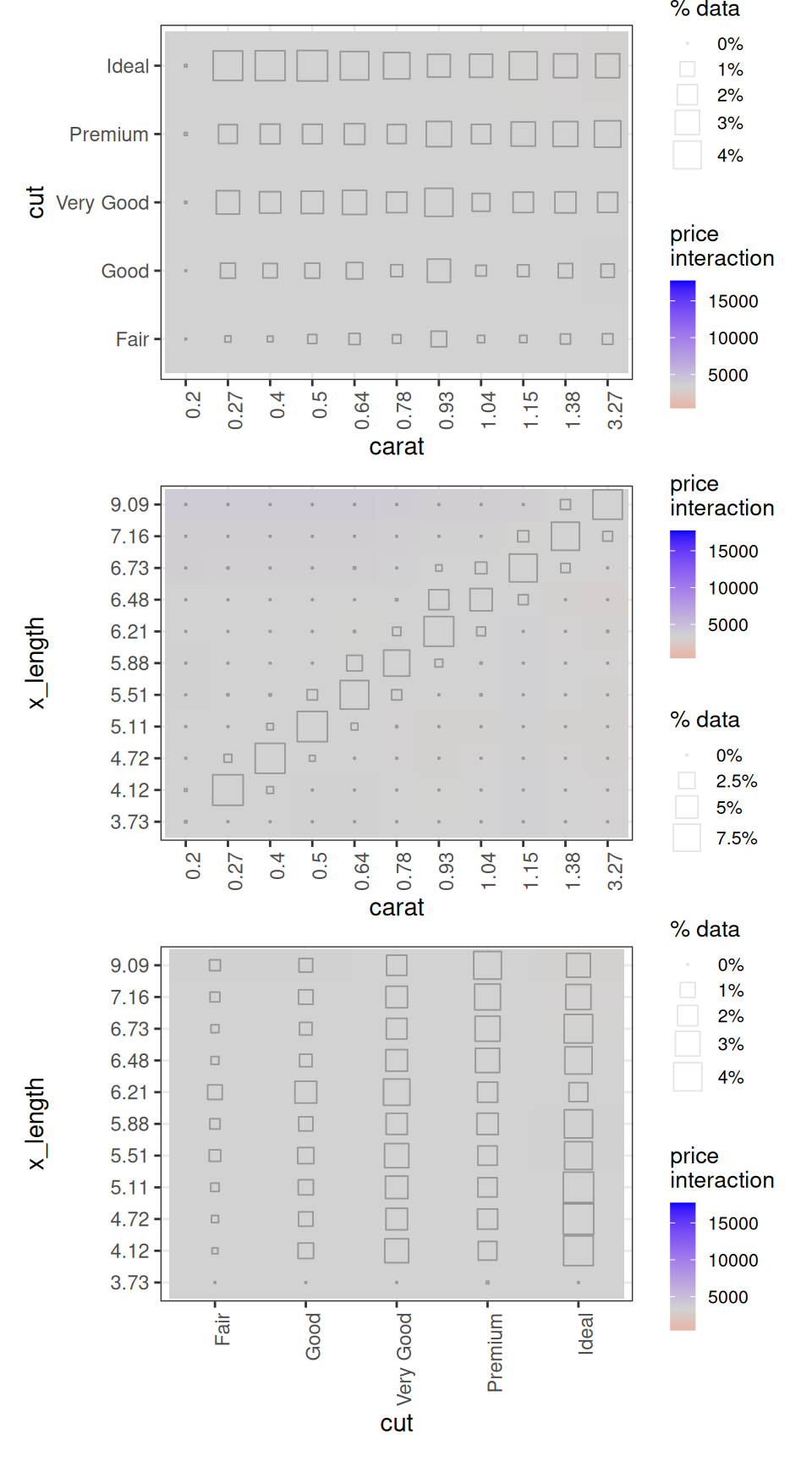
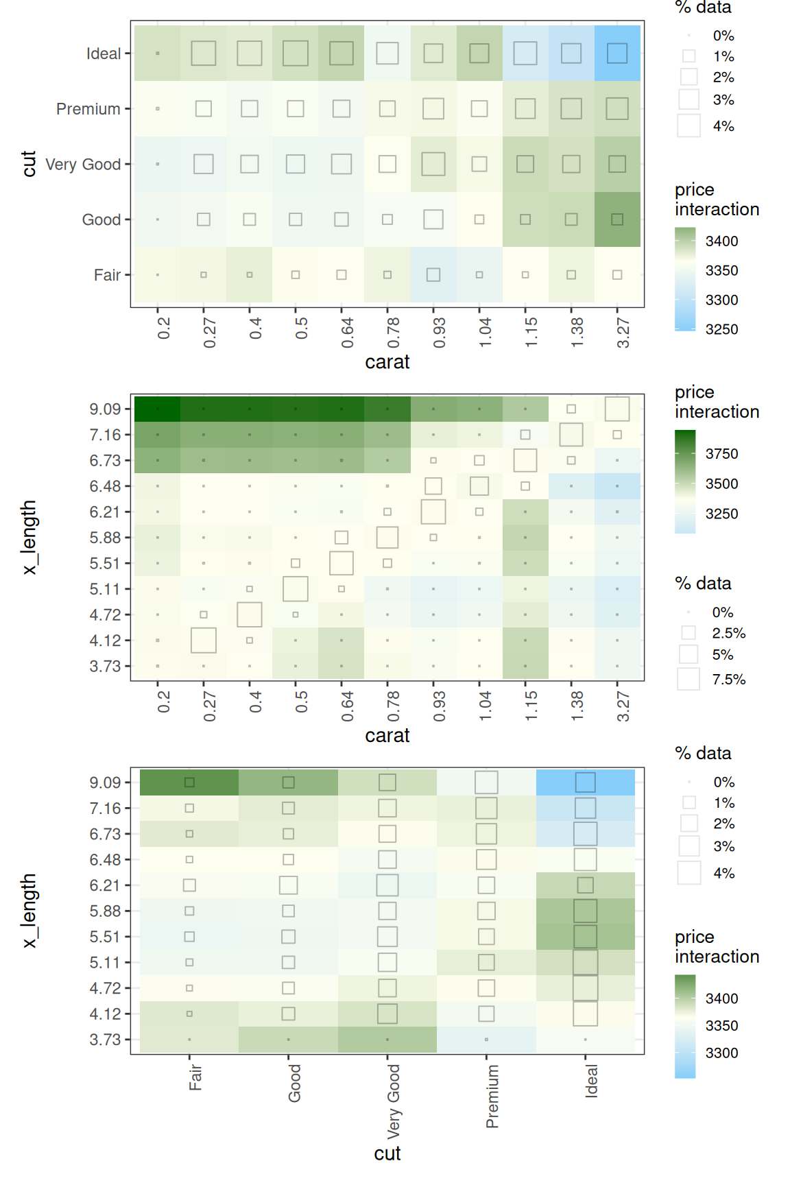
The 2D plots show interaction effects beyond the separate 1D effects. Both axes represent predictors; the fill colour represents the interaction effect on the price scale. The hollow squares indicate the percentage of observations in each combination of bins. See the introductory vignette for their interpretation.
Choose which plots to customize
The x_cols argument of customize() selects the plots to modify. A variable name selects a 1D plot; a term such as "carat:cut" selects an interaction plot. We can use list(d1 = TRUE) or list(d2 = TRUE) to select every available plot of one dimension, or list(d1 = TRUE, d2 = TRUE) to select both dimensions.
Leaving x_cols unspecified applies the customization to all available plots when the object contains only one dimension. When both 1D and 2D plots exist, x_cols must be specified explicitly; it may select either dimension or both.
Because our object contains both 1D and 2D plots, we explicitly specify x_cols in each call to customize(). The following example zooms the y-axis ranges of the 1D carat and cut plots:
selected_plots <- diamonds_plots |>
  customize(
    x_cols = c("carat", "cut"),
    zoom_y = c(1000, 8000)
  )

selected_plots |>
  subset(list(d1 = TRUE)) |>
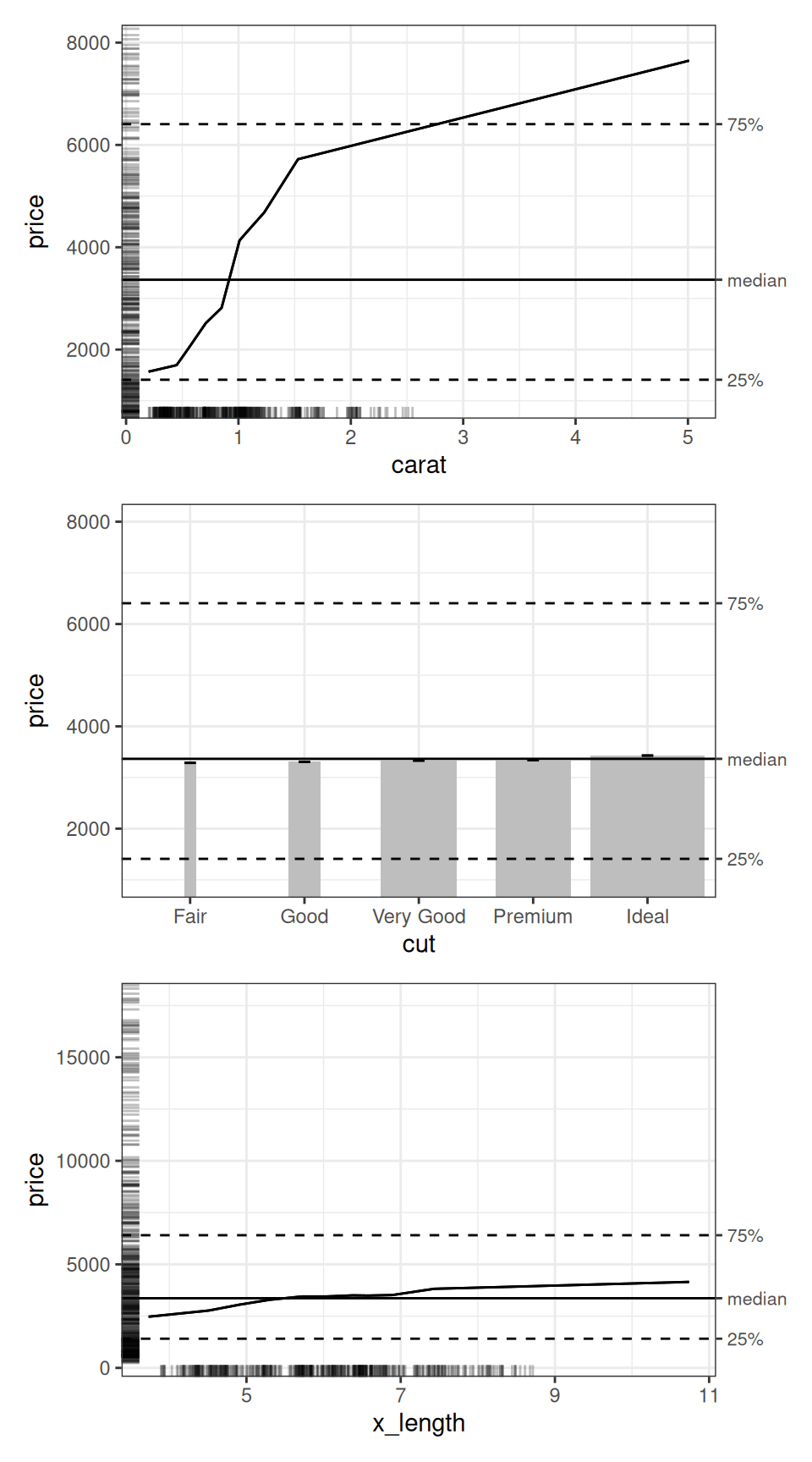
  print(ncol = 1)
The x_length plot retains its original appearance. Customizing plots with customize() does not remove the other plots from the returned object. However, we use subset() to choose which plots to display, excluding the others.
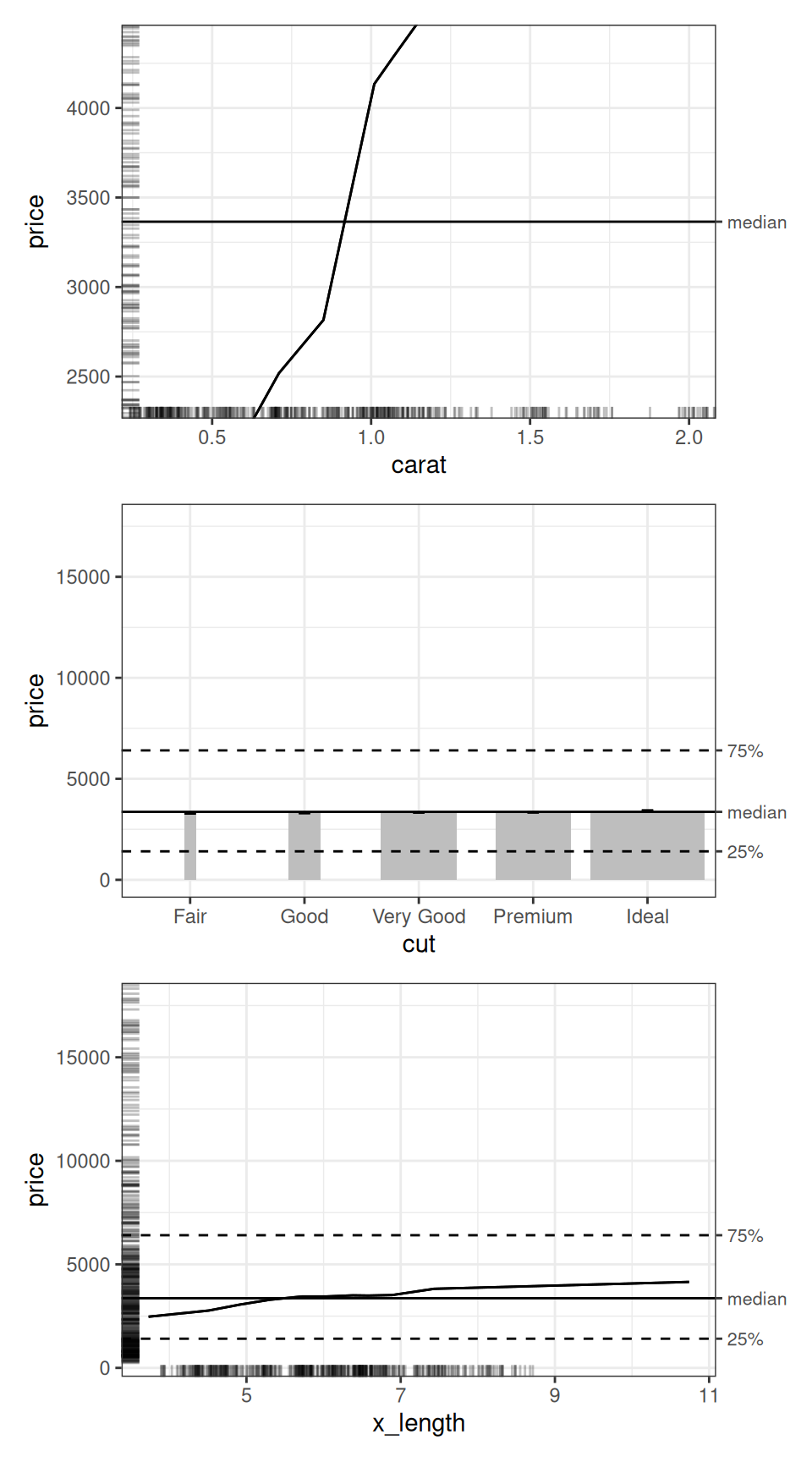
The exclude_cols argument excludes plots from the customization selection. The plots remain unchanged in the ALEPlots object. For example, we can apply the same zoom to every 1D plot except cut:
diamonds_plots |>
  customize(
    x_cols = list(d1 = TRUE),
    exclude_cols = "cut",
    zoom_y = c(1000, 8000)
  ) |>
  subset(list(d1 = TRUE)) |>
  print(nrow = 3)
Here, the change applies to carat and x_length. All six plots are still in numeric_plots. See help(resolve_x_cols) for more selection formats.
Focus on a predictor range with zoom_x
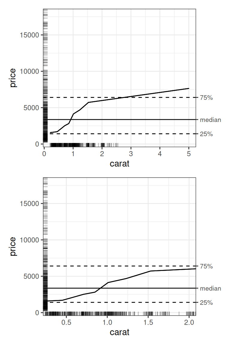
The zoom_x argument of customize() takes a two-element numeric vector giving the lower and upper visible limits of the x-axis. Because our object contains both 1D and 2D plots, we explicitly specify x_cols in each call to customize(). The following example increases the axis text size in the 1D carat and cut plots. The original plot is on top; the zoomed plot is below:
carat_limits <- c(0.3, 2)

x_zoomed_plots <- diamonds_plots |>
  customize(
    x_cols = "carat",
    zoom_x = carat_limits
  )

patchwork::wrap_plots(
  get(diamonds_plots, "carat"),
  get(x_zoomed_plots, "carat"),
  nrow = 2
)
Zooming changes the viewing window, retaining the underlying plotted data. The rug marks help us see where observations lie within the visible range. Values outside this range are still part of the original ALE calculation and can be plotted by respecifying customize().
We apply this numeric x-axis zoom only to the 1D carat plot. Its limits are in carats. The cut plot has discrete levels, and even numeric predictors in 2D plots are displayed as discrete ALE bins, so the same limits would not have the same meaning on the other plots.
Reveal smaller effects with zoom_y
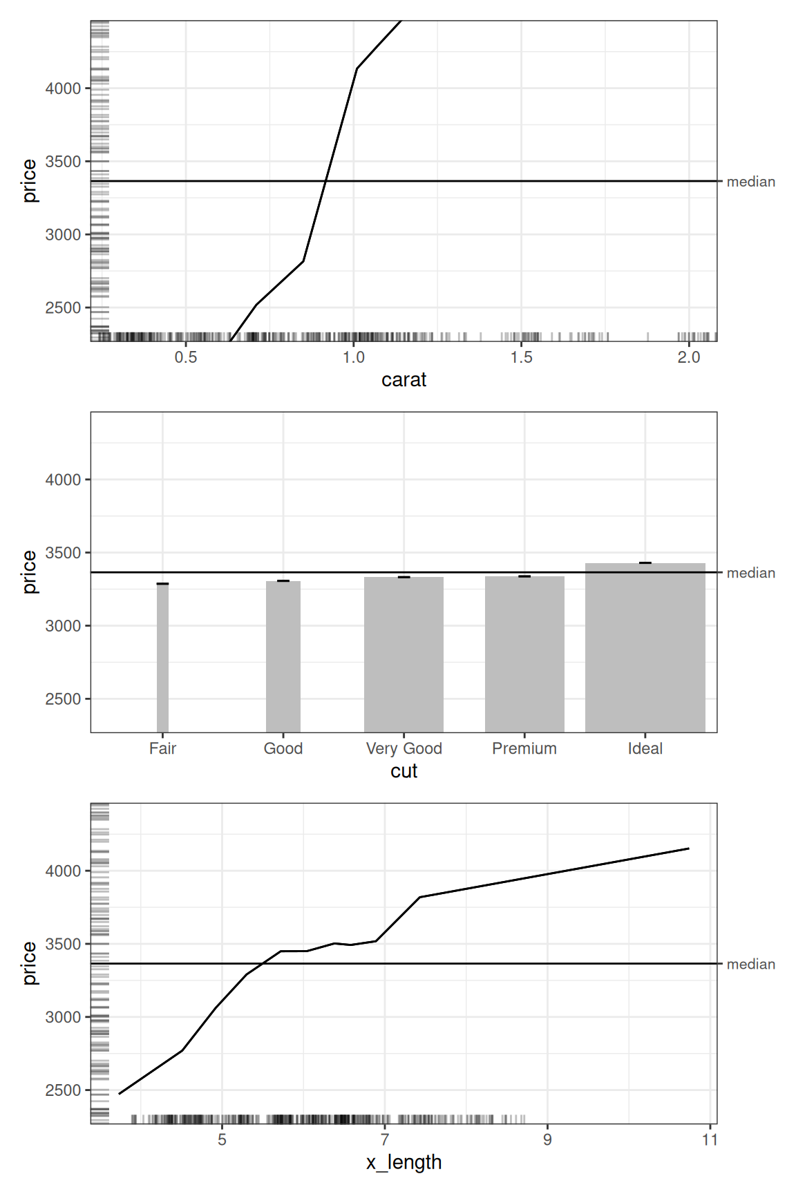
The default y range includes the range of observed diamond prices. This provides context, but smaller effects can be difficult to see. We can narrow the y range for all three 1D variables in a single call with x_cols = list(d1 = TRUE). We use the same limits for each plot to keep their scales comparable:
price_limits <- median(diamonds$price) + c(-1000, 1000)

zoomed_plots <- x_zoomed_plots |>
  customize(
    x_cols = list(d1 = TRUE),
    zoom_y = price_limits
  )

zoomed_plots |>
  subset(list(d1 = TRUE)) |>
  print(ncol = 1)
This makes the differences between cut qualities easier to see. Parts of the carat and x_length curves extend beyond the viewing window. In the column chart, the visible columns also begin above their original zero baseline; we should read the axis values when assessing their differences.
Notice that the carat plot retains the x limits set in the preceding section. Leaving an axis at its default NULL preserves that axis’s existing limits; it does not reset the zoom. The other two 1D plots retain their original x ranges, and the 2D plots retain their original limits.
We can also set both axes in one call:
both_zoomed_plots <- diamonds_plots |>
  customize(
    x_cols = "carat",
    zoom_x = carat_limits,
    zoom_y = price_limits
  )

both_zoomed_plots |>
  subset(list(d1 = TRUE)) |>
  print(ncol = 1)
To zoom out again, supply wider limits. To recover the original view, start from diamonds_plots, which we have kept unchanged.
Flexible customizations with layers
ALE plots in the ale package are implemented with {ggplot2}, so they retain its full flexibility in customization. This flexibility is leveraged through the layers argument of customize(), which accepts a list of additions that ggplot2 supports through its + operator. This includes themes, geometries, and scales. The additions are applied to each selected plot in the order given in the list.
The additions must be appropriate for every selected plot. Shared themes can be applied across dimensions, while scales, coordinates, and geometries may depend on each plot’s axes, mappings, or data. In particular, the y-axis represents the outcome in 1D plots and the second predictor in 2D plots.
Apply a common theme to all plots
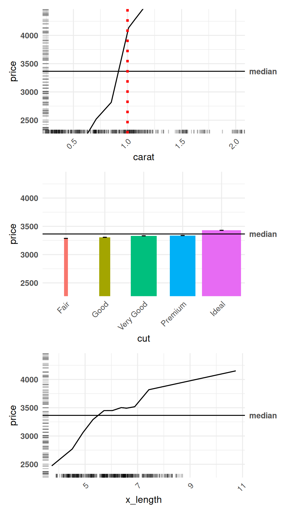
We begin again with the original plots. We can select both dimensions explicitly to apply the same appearance settings to all six plots:
The 2D plots have also received these settings; we will display them after changing their colours below. Keeping the theme settings in a list lets us reuse them in other calls.
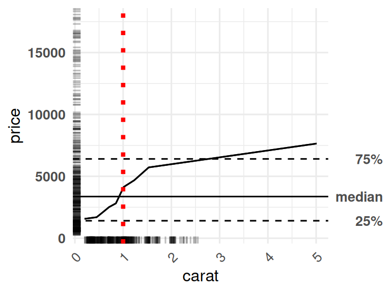
Mark one carat in the 1D carat plot
We add a vertical reference line at one carat. Selecting "carat" applies it only to that 1D plot, leaving interactions involving carat unchanged.
carat_reference <- list(
  geom_vline(
    xintercept = 1,
    colour = "red",
    linetype = "dotted",
    linewidth = 1.5
  )
)

reference_plots <- themed_plots |>
  customize(
    x_cols = "carat",
    layers = carat_reference
  )

get(reference_plots, "carat")
Use the default ggplot colours for cut
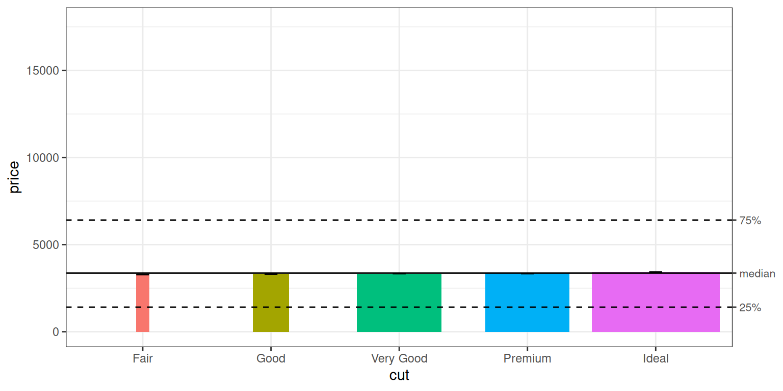
By default, the 1D cut plot draws grey columns. We can set the colours to the {ggplot2} default of using different colours per category simply by adding a ggplot2::scale_fill_discrete() layer:
The colours come from the default discrete fill palette of the active ggplot theme. We use scale_fill_discrete() explicitly because cut is ordered, for which ggplot would otherwise select an ordered palette. Each quality is already identified on the x-axis, so the new columns do not add a fill legend.
Change the colours of all 2D plots
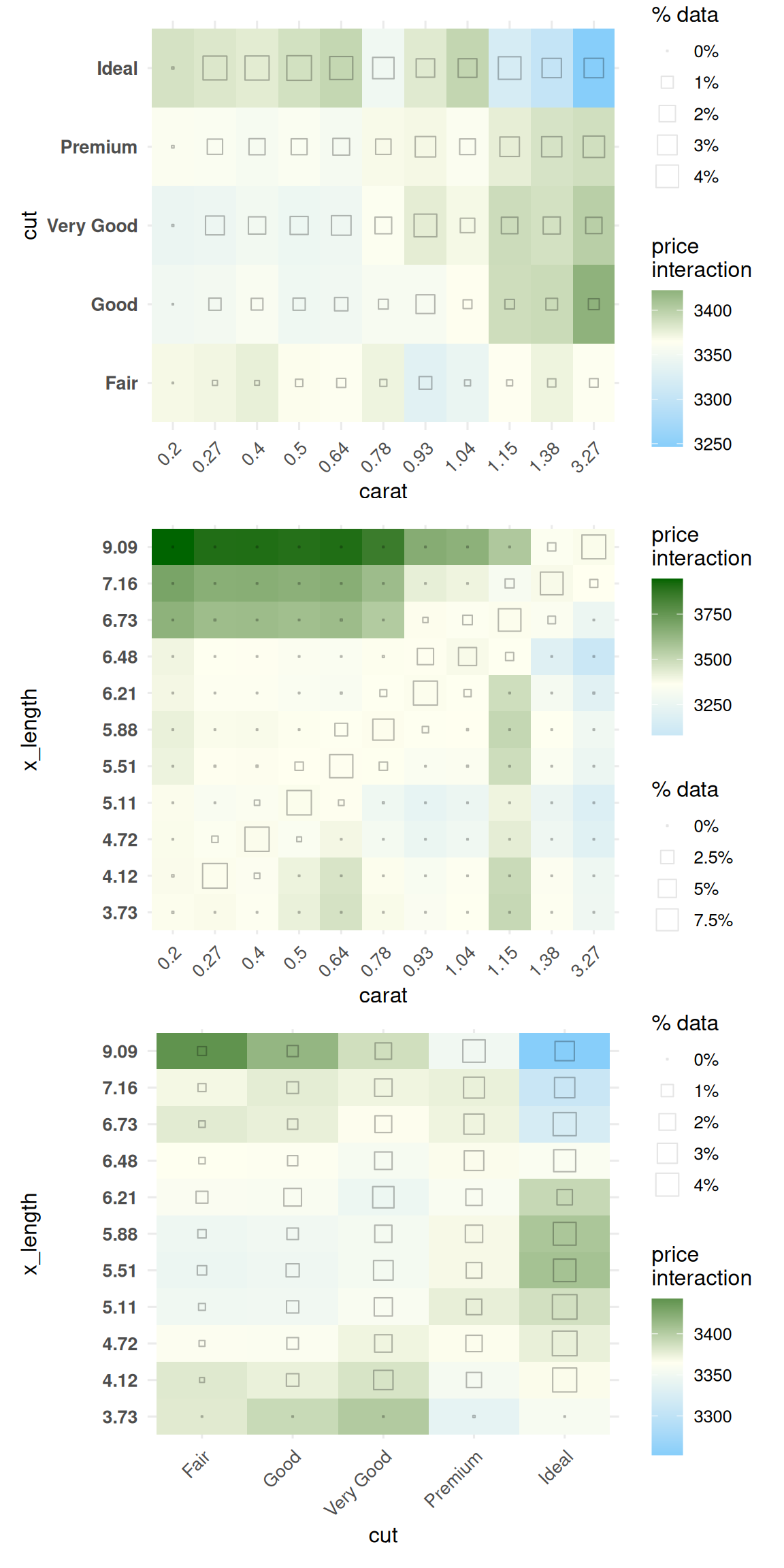
We can replace the red-grey-blue fill scale with a blue-ivory-green scale for all three interaction plots in one call. We keep the midpoint at the median diamond price, matching the default centring of these plots.
interaction_colours <- list(
  scale_fill_gradient2(
    low = "lightskyblue",
    mid = "ivory",
    high = "darkgreen",
    midpoint = median(diamonds$price)
  )
)

interaction_colour_plots <- diamonds_plots |>
  customize(
    x_cols = list(d2 = TRUE),
    layers = interaction_colours
  )

interaction_colour_plots |>
  subset(list(d2 = TRUE)) |>
  print(ncol = 1)
Only the 2D fill scales change; the 1D cut plot retains its discrete colours. The size legends and hollow squares continue to show how much data supports each interaction bin.
When layers and zoom arguments occur in the same call, customize() adds the layers first, then applies the requested zoom. A NULL zoom argument preserves the corresponding limits after the layers have been added. If you need to control the ordering of coordinate changes yourself, supply them only through layers.
Combine the customizations
We can now combine the settings in a pipeline. Starting from the original collection, we apply the common theme to all six plots, zoom the y-axis for all three 1D plots, add the one-carat line and x zoom only to carat, recolour cut, and change the fill scale of all the interactions.
final_plots <- diamonds_plots |>
  customize(
    x_cols = list(d1 = TRUE, d2 = TRUE),
    layers = common_theme
  ) |>
  customize(
    x_cols = list(d1 = TRUE),
    zoom_y = price_limits
  ) |>
  customize(
    x_cols = "carat",
    layers = carat_reference,
    zoom_x = carat_limits
  ) |>
  customize(
    x_cols = "cut",
    layers = cut_colours
  ) |>
  customize(
    x_cols = list(d2 = TRUE),
    layers = interaction_colours
  )

final_plots |>
  subset(list(d1 = TRUE)) |>
  print(ncol = 1)
The main arguments demonstrated in this article are:
x_cols |
Select the variables or interactions whose plots should change. |
exclude_cols |
Exclude plots from that selection. |
zoom_x |
Set the visible x range of the selected plots. |
zoom_y |
Set the visible y range of the selected plots. |
layers |
Append ggplot additions to each selected plot. |
See help(customize) for the full function reference and help(ALEPlots) for options available when first generating plots.